Calculating the SNR associated with an astrophysical signal model

The example Filtering a TimeSeries to detect gravitational waves showed us we can visually extract a signal from the noise using basic signal-processing techniques.

However, an actual astrophysical search algorithm detects signals by calculating the signal-to-noise ratio (SNR) of data for each in a large bank of signal models, known as templates.

Using PyCBC (the actual search code), we can do that.

Data access and conditioning

First we fetch some of the public data from GWOSC:

from gwpy.timeseries import TimeSeries
data = TimeSeries.get("H1", 1126259446, 1126259478)

and condition it by applying a highpass filter at 15 Hz

high = data.highpass(15)

This is important to remove noise at lower frequencies that isn’t accurately calibrated, and swamps smaller noises at higher frequencies.

For this example, we want to calculate the SNR over a 4 second segment, so we calculate a Power Spectral Density with a 4 second FFT length (using all of the data), then crop() the data:

psd = high.psd(4, 2)
zoom = high.crop(1126259460, 1126259464)

Generating a signal model

In order to calculate signal-to-noise ratio, we need a signal model against which to compare our data. For this we import pycbc.waveform.get_fd_waveform and generate a template as a pycbc.types.FrequencySeries:

from pycbc.waveform import get_fd_waveform
hp, _ = get_fd_waveform(
    approximant="IMRPhenomD",
    mass1=40,
    mass2=32,
    f_lower=20,
    f_final=2048,
    delta_f=psd.df.value,
)

/home/docs/checkouts/readthedocs.org/user_builds/gwpy/conda/latest/lib/python3.12/site-packages/pycbc/waveform/nltides.py:13: SyntaxWarning: invalid escape sequence '\p'
  Delta Psi(f) = 2 \pi f Delta t(f) - Delta phi(f)
/home/docs/checkouts/readthedocs.org/user_builds/gwpy/conda/latest/lib/python3.12/site-packages/pycbc/tmpltbank/calc_moments.py:333: SyntaxWarning: invalid escape sequence '\i'
  \int funct(x) * (psd_x)**(-7./3.) * delta_x / PSD(x)
/home/docs/checkouts/readthedocs.org/user_builds/gwpy/conda/latest/lib/python3.12/site-packages/pycbc/tmpltbank/option_utils.py:177: SyntaxWarning: invalid escape sequence '\i'
  "space metric:  integrals of the form \int F(f) df "
/home/docs/checkouts/readthedocs.org/user_builds/gwpy/conda/latest/lib/python3.12/site-packages/pycbc/tmpltbank/option_utils.py:178: SyntaxWarning: invalid escape sequence '\s'
  "are approximated as \sum F(f) delta_f.  REQUIRED. "

Calculating SNR

At this point we are ready to calculate the SNR, so we import the pycbc.filter.matched_filter method, and pass it our template, the data, and the PSD:

from pycbc.filter import matched_filter
snr = matched_filter(
    hp,
    zoom.to_pycbc(),
    psd=psd.to_pycbc(),
    low_frequency_cutoff=15,
)
snrts = TimeSeries.from_pycbc(snr).abs()

Tip

Here we have used the to_pycbc() methods of the TimeSeries and FrequencySeries objects to convert from GWpy objects to something that PyCBC functions can understand, and then used the from_pycbc() method to convert back to a GWpy object.

Visualisation

We can plot the SNR TimeSeries around the region of interest:

plot = snrts.plot()
ax = plot.gca()
ax.set_xlim(1126259461, 1126259463)
ax.set_epoch(1126259462.427)
ax.set_ylabel("Signal-to-noise ratio (SNR)")
ax.set_title("LIGO-Hanford signal-correlation for GW150914")
plot.show()

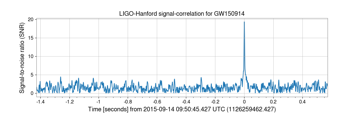
We can clearly see a large spike (above 17!) at the time of the GW150914 signal! This is, in principle, how the full, blind, CBC search is performed, using all of the available data, and a bank of tens of thousand of signal models.