Calculate the coherence between two channels

The coherence between two channels is a measure of the frequency-domain correlation between their time-series data.

In LIGO, the coherence is a crucial indicator of how noise sources couple into the main differential arm-length readout. Here we use use the TimeSeries.coherence() method to highlight coupling of the mains power supply into the strain output of the LIGO-Hanford interferometer.

These data are available as part of the O3 Auxiliary Channel Data Release.

Data access

First, we import the TimeSeries

from gwpy.timeseries import TimeSeries

and then get() the LIGO-Hanford strain data, and the mains power monitor data, for a 600-second window near the end of the O3 Auxiliary Channel Data Release:

start = 1389410000
end = 1389410600
strain = TimeSeries.get("H1", start, end)
mains = TimeSeries.get(
    "H1:PEM-EY_MAINSMON_EBAY_1_DQ",
    start,
    end,
    frametype="H1_AUX_AR1",
)

Data are accessed separately

We could have used TimeSeriesDict.get to access both channels in a single call - that method would first try to find a single dataset that contain both of them, then automatically fall back to separate calls if that fails.

But, since we know that these channels are in different datsets, we access them separately here for clarity and speed.

Calculating coherence

We can then calculate the coherence() of one TimeSeries with respect to the other, using an 8-second Fourier transform length, with a 4-second (50%) overlap:

coh = strain.coherence(mains, fftlength=8, overlap=4)

/home/docs/checkouts/readthedocs.org/user_builds/gwpy/checkouts/stable/gwpy/signal/spectral/_ui.py:356: UserWarning: Sampling frequencies are unequal. Higher frequency series will be downsampled before coherence is calculated
  return method_func(

The output of this method is a FrequencySeries containing the coherence values for each frequency bin.

Visualisation

We can now plot() the coherence:

plot = coh.plot(
    xlabel="Frequency [Hz]",
    xscale="log",
    ylabel="Coherence",
    yscale="linear",
    ylim=(0, 1),
)
plot.show()

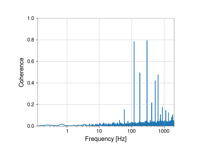
Here we can see strong coherence at 60 Hz and its harmonics, indicating that the mains power supply is coupling into the differential arm length control loop.