Visualising filters (BodePlot)#
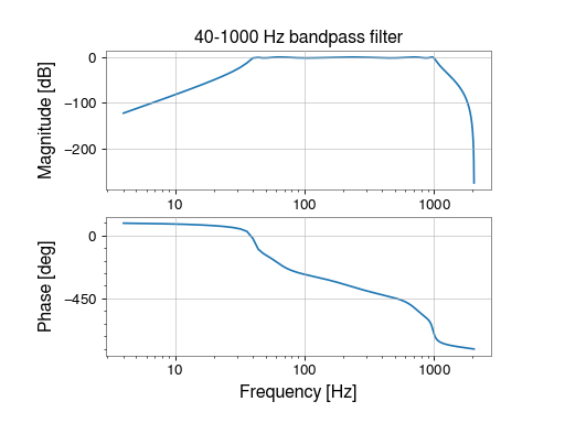
Any time-domain or Fourier-domain filters can be visualised using the Bode plot,
showing the magnitude (in decibels) and phase (in degrees) response of a linear time-invariant filter.
The BodePlot allows for simple display of these responses for any filter,
for example a 40-1000 Hertz band-pass filter to be applied to a digital signal sampled at 4096 Hertz:
>>> from gwpy.signal.filter_design import bandpass
>>> from gwpy.plot import BodePlot
>>> zpk = bandpass(40, 1000, 4096)
>>> plot = BodePlot(zpk, sample_rate=4096, title='40-1000 Hz bandpass filter')
>>> plot.show()
(png)
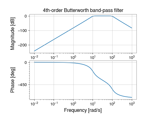
The BodePlot also supports visualising analogue filters,
for example a 4th-order Butterworth band-pass filter.
>>> from scipy.signal import butter
>>> from gwpy.plot import BodePlot
>>> zpk = butter(4, (10, 100), btype="bandpass", analog=True)
>>> plot = BodePlot(zpk, title='4th-order Butterworth band-pass filter', analog=True)
>>> plot.show()
(png)