Calculate and plot a FrequencySeries

One of the principal means of estimating the sensitivity of a gravitational-wave detector is to esimate it’s amplitude spectral density (ASD). The ASD is a measurement of how a signal’s amplitude varies across different frequencies.

The ASD can be estimated directly from a TimeSeries using the asd() method.

Data access

For this example we choose to estimate the ASD around GW200115, one of the first observations of a neutron star-black hole binary. We can use the gwosc Python package to query for the relevant GPS time:

from gwosc.datasets import event_gps

gps = event_gps("GW200115")

In order to generate a FrequencySeries we need to import the TimeSeries and use fetch_open_data() to download the strain records:

from gwpy.timeseries import TimeSeries

lho = TimeSeries.get("H1", gps - 16, gps + 16)
llo = TimeSeries.get("L1", gps - 16, gps + 16)

Calculate the ASDs

We can then call the asd() method to calculated the amplitude spectral density for each TimeSeries:

lhoasd = lho.asd(4, 2)
lloasd = llo.asd(4, 2)

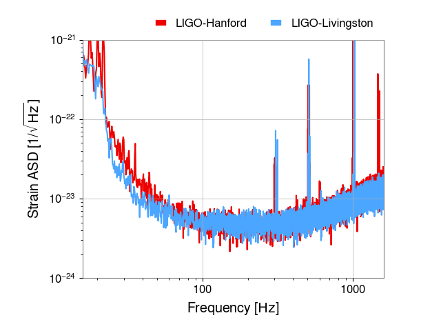
Visualisation

We can then plot() the spectra using the ‘standard’ colour scheme:

plot = lhoasd.plot(label="LIGO-Hanford", color="gwpy:ligo-hanford")
ax = plot.gca()
ax.plot(lloasd, label="LIGO-Livingston", color="gwpy:ligo-livingston")
ax.set_xlim(16, 1600)
ax.set_ylim(1e-24, 1e-21)
ax.set_ylabel(r"Strain ASD [1/$\sqrt{\mathrm{Hz}}]$")
ax.legend(frameon=False, bbox_to_anchor=(1., 1.), loc="lower right", ncol=2)
plot.show()