TimeSeries#

Bases: TimeSeriesBase

A time-domain data array.

Parameters:

valuearray_like: Input data array.
unitUnit, optional: Physical unit of these data.
t0LIGOTimeGPS, float, str, optional: GPS epoch associated with these data, any input parsable by to_gps is fine.
dtfloat, Quantity, optional: Time between successive samples (seconds), can also be given inversely via sample_rate.
sample_ratefloat, Quantity, optional: The rate of samples per second (Hertz), can also be given inversely via dt.
timesarray-like: The complete array of GPS times accompanying the data for this series. This argument takes precedence over t0 and dt so should be given in place of these if relevant, not alongside.
namestr, optional: Descriptive title for this array.
channelChannel, str, optional: Source data stream for these data.
dtypedtype, optional: Input data type.
copybool, optional: Choose to copy the input data to new memory.
subokbool, optional: Allow passing of sub-classes by the array generator.

Notes

The necessary metadata to reconstruct timing information are recorded in the epoch and sample_rate attributes. This time-stamps can be returned via the times property.

All comparison operations performed on a TimeSeries will return a StateTimeSeries - a boolean array with metadata copied from the starting TimeSeries.

Examples

>>> from gwpy.timeseries import TimeSeries

To create an array of random numbers, sampled at 100 Hz, in units of ‘metres’:

>>> from numpy import random
>>> series = TimeSeries(random.random(1000), sample_rate=100, unit='m')

which can then be simply visualised via

>>> plot = series.plot()
>>> plot.show()

(png)

../../_images/gwpy-timeseries-TimeSeries-1.png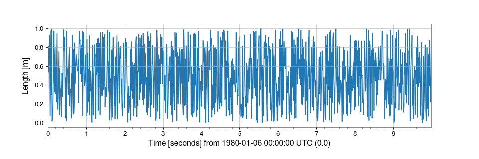

Attributes Summary

`get`	Retrieve data for a channel from any data source.
`read`	Read data into a `TimeSeries`.
`write`	Write this `TimeSeries` to a file.

Methods Summary

`asd`([fftlength, overlap, window, method])	Calculate the ASD `FrequencySeries` of this `TimeSeries`.
`auto_coherence`(dt[, fftlength, overlap, window])	Calculate the coherence between this series and a shifted copy of itself.
`average_fft`([fftlength, overlap, window])	Compute the averaged one-dimensional DFT of this `TimeSeries`.
`bandpass`(flow, fhigh[, gpass, gstop, fstop, ...])	Filter this `TimeSeries` with a band-pass filter.
`coherence`(other[, fftlength, overlap, window])	Calculate the frequency-coherence between this `TimeSeries` and another.
`coherence_spectrogram`(other, stride[, ...])	Calculate the coherence spectrogram between this `TimeSeries` and other.
`convolve`(fir[, window])	Convolve this `TimeSeries` with an FIR filter using the overlap-save method.
`correlate`(mfilter[, window, detrend, ...])	Cross-correlate this `TimeSeries` with another signal.
`csd`(other[, fftlength, overlap, window])	Calculate the CSD `FrequencySeries` for two `TimeSeries`.
`csd_spectrogram`(other, stride[, fftlength, ...])	Calculate the cross spectral density spectrogram with `other`.
`demodulate`(...)	Compute the average magnitude and phase of this `TimeSeries`.
`detrend`([detrend])	Remove the trend from this `TimeSeries`.
`fft`([nfft])	Compute the one-dimensional discrete Fourier transform of this `TimeSeries`.
`fftgram`(fftlength[, overlap, window])	Calculate the Fourier-gram of this `TimeSeries`.
`filter`(filt, *[, analog, unit, ...])	Filter this `TimeSeries` with an IIR or FIR filter.
`find_gates`([tzero, whiten, threshold, ...])	Identify points that should be gates using a provided threshold.
`gate`([tzero, tpad, whiten, threshold, ...])	Remove high amplitude peaks from data using inverse Tukey window.
`heterodyne`(phase[, stride, singlesided])	Compute the heterodyned average magnitude and phase of this `TimeSeries`.
`highpass`(frequency[, gpass, gstop, fstop, ...])	Filter this `TimeSeries` with a high-pass filter.
`lowpass`(frequency[, gpass, gstop, fstop, ...])	Filter this `TimeSeries` with a Butterworth low-pass filter.
`mask`([deadtime, flag, query_open_data, ...])	Mask portions of this `TimeSeries` that fall within a given list of segments.
`notch`(frequency[, type, filtfilt])	Notch out a frequency in this `TimeSeries`.
`psd`([fftlength, overlap, window, method])	Calculate the PSD `FrequencySeries` for this `TimeSeries`.
`q_gram`([qrange, frange, mismatch, snrthresh])	Scan a `TimeSeries` using the multi-Q transform.
`q_transform`([qrange, frange, gps, search, ...])	Compute the multi-Q transform and return an interpolated spectrogram.
`rayleigh_spectrogram`(stride[, fftlength, ...])	Calculate the Rayleigh statistic spectrogram of this `TimeSeries`.
`rayleigh_spectrum`([fftlength, overlap, window])	Calculate the Rayleigh `FrequencySeries` for this `TimeSeries`.
`resample`(rate[, window, ftype, n])	Resample this Series to a new rate.
`rms`([stride])	Calculate the root-mean-square value of this `TimeSeries` once per stride.
`spectral_variance`(stride[, fftlength, ...])	Calculate the `SpectralVariance` of this `TimeSeries`.
`spectrogram`(stride[, fftlength, overlap, ...])	Calculate the average power spectrogram of this `TimeSeries`.
`spectrogram2`(fftlength[, overlap, window])	Calculate the non-averaged power `Spectrogram` of this `TimeSeries`.
`taper`([side, duration, nsamples])	Taper the ends of this `TimeSeries` smoothly to zero.
`transfer_function`(other[, fftlength, ...])	Calculate the transfer function between this `TimeSeries` and another.
`whiten`([fftlength, overlap, method, window, ...])	Whiten this `TimeSeries` using inverse spectrum truncation.
`zpk`(zeros, poles, gain, *[, analog, unit, ...])	Filter this `TimeSeries` by applying a digital zero-pole-gain filter.

Attributes Documentation

get#

Retrieve data for a channel from any data source.

This method attempts to get data any way it can, potentially iterating over multiple available data sources.

Parameters:

channelslist

Required data channels.

startLIGOTimeGPS, float, str

GPS start time of required data, any input parseable by to_gps is fine

endLIGOTimeGPS, float, str

GPS end time of required data, any input parseable by to_gps is fine

sourcestr, list, list of dict.

The data source to use. One of the following formats:

str - the name of a single source to use,
list - a list of source names to try in order,
list of dict - a list of source specifications to try in order; each dict must contain a "source" key giving the name of the source to use, and may contain other keys giving options to pass to the data access function for that source.

See ‘Notes’ section below for valid source names.

frametypestr

Name of frametype in which this channel is stored, by default will search for all required frame types.

padfloat

Value with which to fill gaps in the source data, by default gaps will result in a ValueError.

scaledbool

apply slope and bias calibration to ADC data, for non-ADC data this option has no effect.

nprocint, default: 1

Number of parallel processes to use, serial process by default.

allow_tapebool, default: None

Allow the use of data files that are held on tape. Default is None to attempt to allow the TimeSeries.fetch method to intelligently select a server that doesn’t use tapes for data storage (doesn’t always work), but to eventually allow retrieving data from tape if required.

verbosebool

This argument is deprecated and will be removed in a future release. Use DEBUG-level logging instead, see Logging with GWpy.

kwargs

Other keyword arguments to pass to the data access function for each data source.

read#

Read data into a TimeSeries.

Arguments and keywords depend on the output format, see the online documentation for full details for each format, the parameters below are common to all formats.

Parameters:

sourcestr, os.PathLike, file, or list of these

Source of data, any of the following:

Path of a single data file
List of data file paths
Path of LAL-format cache file

namestr, optional

The name of the data object to read, or a Channel object. This argument is required if source contains (or may contain) multiple datasets.

When reading from GWF, this argument should specify the name of the channel to read.
When reading from HDF5, this argument should specify the path or dataset name within the file.

startLIGOTimeGPS, float, str, optional

GPS start time of required data, defaults to start of data found; any input parseable by to_gps is fine.

endLIGOTimeGPS, float, str, optional

GPS end time of required data, defaults to end of data found; any input parseable by to_gps is fine.

formatstr, optional

Source format identifier. If not given, the format will be detected if possible. See below for list of acceptable formats.

parallelint, optional

Number of parallel processes to use, serial process by default.

padfloat, optional

Value with which to fill gaps in the source data, by default gaps will result in a ValueError.

Raises:

IndexError: if source is an empty list

write#

Write this TimeSeries to a file.

Arguments and keywords depend on the output format, see the online documentation for full details for each format, the parameters below are common to most formats.

Parameters:

targetstr: output filename
formatstr, optional: output format identifier. If not given, the format will be detected if possible. See below for list of acceptable formats.

Methods Documentation

asd(

fftlength: float | None = None,

overlap: float | None = None,

window: WindowLike = 'hann',

method: str = 'median',

**kwargs,

) → FrequencySeries[source]#

Calculate the ASD FrequencySeries of this TimeSeries.

Parameters:

fftlengthfloat: Number of seconds in single FFT, defaults to a single FFT covering the full duration.
overlapfloat, optional: Number of seconds of overlap between FFTs, defaults to the recommended overlap for the given window (if given), or 0.
windowstr, numpy.ndarray, optional: Window function to apply to timeseries prior to FFT, see scipy.signal.get_window() for details on acceptable formats.
methodstr, optional: FFT-averaging method (default: 'median'), see Notes for more details
kwargs: Other keyword arguments are passed to the underlying ASD-generation method.

Returns:

asdFrequencySeries: A data series containing the ASD.

See also

TimeSeries.psd

Notes

The accepted method arguments are:

'bartlett' : a mean average of non-overlapping periodograms
'median' : a median average of overlapping periodograms
'welch' : a mean average of overlapping periodograms

auto_coherence(

dt: float,

fftlength: float | None = None,

overlap: float | None = None,

window: WindowLike = 'hann',

**kwargs,

) → FrequencySeries[source]#

Calculate the coherence between this series and a shifted copy of itself.

The standard TimeSeries.coherence() is calculated between the input TimeSeries and a cropped copy of itself. Since the cropped version will be shorter, the input series will be shortened to match.

Parameters:

dtfloat: Duration (in seconds) of time-shift.
fftlengthfloat, optional: Number of seconds in single FFT, defaults to a single FFT covering the full duration.
overlapfloat, optional: Number of seconds of overlap between FFTs, defaults to the recommended overlap for the given window (if given), or 0.
windowstr, numpy.ndarray, optional: Window function to apply to timeseries prior to FFT, see scipy.signal.get_window() for details on acceptable formats.
kwargs: Any other keyword arguments accepted by matplotlib.mlab.cohere() except NFFT, window, and noverlap which are superceded by the above keyword arguments.

Returns:

coherenceFrequencySeries: The coherence FrequencySeries of this TimeSeries with the other.

See also

matplotlib.mlab.cohere: For details of the coherence calculator.

Notes

The TimeSeries.auto_coherence() will perform best when dt is approximately fftlength / 2.

average_fft( fftlength: float | Quantity | None = None, overlap: float | Quantity = 0, window: WindowLike | None = None, ) → FrequencySeries[source]#

Compute the averaged one-dimensional DFT of this TimeSeries.

This method computes a number of FFTs of duration fftlength and overlap (both given in seconds), and returns the mean average. This method is analogous to the Welch average method for power spectra.

Parameters:

fftlengthfloat: Number of seconds in single FFT; by default uses whole TimeSeries.
overlapfloat, optional: Number of seconds of overlap between FFTs, defaults to the recommended overlap for the given window (if given), or 0.
windowstr, numpy.ndarray, optional: Window function to apply to timeseries prior to FFT, see scipy.signal.get_window() for details on acceptable formats.

Returns:

outcomplex-valued FrequencySeries: The transformed output, with populated frequencies array metadata.

See also

TimeSeries.fft: The FFT method used.

bandpass(

flow: float,

fhigh: float,

gpass: float = 2,

gstop: float = 30,

fstop: tuple[float, float] | None = None,

type: Literal['fir', 'iir'] = 'iir',

*,

filtfilt: bool = True,

**kwargs,

) → TimeSeries[source]#

Filter this TimeSeries with a band-pass filter.

Parameters:

flowfloat: Lower corner frequency of pass band.
fhighfloat: Upper corner frequency of pass band.
gpassfloat: The maximum loss in the passband (dB).
gstopfloat: The minimum attenuation in the stopband (dB).
fstoptuple of float, optional: (low, high) edge-frequencies of stop band.
typestr: The filter type, either 'iir' or 'fir'.
filtfiltbool, optional: If True, apply the filter using a forward-backward filter design, otherwise apply the filter in a single pass. Defaults to True.
kwargs: Other keyword arguments are passed to gwpy.signal.filter_design.bandpass()

Returns:

bpseriesTimeSeries: A band-passed version of the input TimeSeries.

See also

gwpy.signal.filter_design.bandpass: For details on the filter design.
TimeSeries.filter: For details on how the filter is applied.

coherence(

other: TimeSeries,

fftlength: float | None = None,

overlap: float | None = None,

window: WindowLike = 'hann',

**kwargs,

) → FrequencySeries[source]#

Calculate the frequency-coherence between this TimeSeries and another.

Parameters:

otherTimeSeries: TimeSeries signal to calculate coherence with
fftlengthfloat, optional: Number of seconds in single FFT, defaults to a single FFT covering the full duration.
overlapfloat, optional: Number of seconds of overlap between FFTs, defaults to the recommended overlap for the given window (if given), or 0.
windowstr, numpy.ndarray, optional: Window function to apply to timeseries prior to FFT, see scipy.signal.get_window() for details on acceptable formats.
kwargs: Any other keyword arguments accepted by matplotlib.mlab.cohere() except NFFT, window, and noverlap which are superceded by the above keyword arguments.

Returns:

coherenceFrequencySeries: The coherence FrequencySeries of this TimeSeries with the other.

See also

scipy.signal.coherence: For details of the coherence calculator.

Notes

If self and other have difference TimeSeries.sample_rate values, the higher sampled TimeSeries will be down-sampled to match the lower.

coherence_spectrogram( other: TimeSeries, stride: float, fftlength: float | None = None, overlap: float | None = None, window: WindowLike = 'hann', nproc: int = 1, ) → Spectrogram[source]#

Calculate the coherence spectrogram between this TimeSeries and other.

Parameters:

otherTimeSeries: The second TimeSeries in this CSD calculation.
stridefloat: Number of seconds in single PSD (column of spectrogram).
fftlengthfloat: Number of seconds in single FFT.
overlapfloat, optional: Number of seconds of overlap between FFTs, defaults to the recommended overlap for the given window (if given), or 0.
windowstr, numpy.ndarray, optional: Window function to apply to timeseries prior to FFT, see scipy.signal.get_window() for details on acceptable formats.
nprocint: Number of parallel processes to use when calculating individual coherence spectra.

Returns:

spectrogramSpectrogram: Time-frequency coherence spectrogram as generated from the input time-series.

convolve(fir: numpy.ndarray, window: WindowLike = 'hann') → Self[source]#

Convolve this TimeSeries with an FIR filter using the overlap-save method.

Parameters:

firnumpy.ndarray: The time domain filter to convolve with.
windowstr, optional: Window function to apply to boundaries, default: 'hann' see scipy.signal.get_window() for details on acceptable formats.

Returns:

outTimeSeries: The result of the convolution.

See also

scipy.signal.fftconvolve: For details on the convolution scheme used here.
TimeSeries.filter: For an alternative method designed for short filters.

Notes

The output TimeSeries is the same length and has the same timestamps as the input.

Due to filter settle-in, a segment half the length of fir will be corrupted at the left and right boundaries. To prevent spectral leakage these segments will be windowed before convolving.

correlate(

mfilter: TimeSeries,

window: WindowLike = 'hann',

detrend: Literal['linear', 'constant'] = 'linear',

*,

whiten: bool = False,

wduration: float = 2,

highpass: float | None = None,

**asd_kw,

) → TimeSeries[source]#

Cross-correlate this TimeSeries with another signal.

Parameters:

mfilterTimeSeries: the time domain signal to correlate with
windowstr, optional: window function to apply to timeseries prior to FFT, default: 'hann' see scipy.signal.get_window() for details on acceptable formats
detrendstr, optional: type of detrending to do before FFT (see detrend for more details), default: 'linear'
whitenbool, optional: boolean switch to enable (True) or disable (False) data whitening, default: False
wdurationfloat, optional: duration (in seconds) of the time-domain FIR whitening filter, only used if whiten=True, defaults to 2 seconds
highpassfloat, optional: highpass corner frequency (in Hz) of the FIR whitening filter, only used if whiten=True, default: None
**asd_kw: keyword arguments to pass to TimeSeries.asd to generate an ASD, only used if whiten=True

Returns:

snrTimeSeries: the correlated signal-to-noise ratio (SNR) timeseries

See also

TimeSeries.asd: for details on the ASD calculation
TimeSeries.convolve: for details on convolution with the overlap-save method

Notes

The window argument is used in ASD estimation, whitening, and preventing spectral leakage in the output. It is not used to condition the matched-filter, which should be windowed before passing to this method.

Due to filter settle-in, a segment half the length of mfilter will be corrupted at the beginning and end of the output. See convolve for more details.

The input and matched-filter will be detrended, and the output will be normalised so that the SNR measures number of standard deviations from the expected mean.

csd(

other: TimeSeries,

fftlength: float | None = None,

overlap: float | None = None,

window: WindowLike = 'hann',

**kwargs,

) → FrequencySeries[source]#

Calculate the CSD FrequencySeries for two TimeSeries.

Parameters:

otherTimeSeries: The second TimeSeries in this CSD calculation.
fftlengthfloat: Number of seconds in single FFT, defaults to a single FFT covering the full duration.
overlapfloat, optional: Number of seconds of overlap between FFTs, defaults to the recommended overlap for the given window (if given), or 0.
windowstr, numpy.ndarray, optional: Window function to apply to timeseries prior to FFT, see scipy.signal.get_window() for details on acceptable formats.
kwargs: Other keyword arguments are passed to the underlying CSD-generation method.

Returns:

csdFrequencySeries: A data series containing the CSD.

csd_spectrogram(

other: TimeSeries,

stride: float,

fftlength: float | None = None,

overlap: float = 0,

window: WindowLike = 'hann',

nproc: int = 1,

**kwargs,

) → Spectrogram[source]#

Calculate the cross spectral density spectrogram with other.

Parameters:

otherTimeSeries: Second time-series for cross spectral density calculation.
stridefloat: Number of seconds in single PSD (column of spectrogram).
fftlengthfloat: Number of seconds in single FFT.
overlapfloat, optional: Number of seconds of overlap between FFTs, defaults to the recommended overlap for the given window (if given), or 0.
windowstr, numpy.ndarray, optional: Window function to apply to timeseries prior to FFT, see scipy.signal.get_window() for details on acceptable formats.
nprocint: Maximum number of independent frame reading processes, default is set to single-process file reading.
kwargs: Other keyword arguments are passed to the underlying CSD-generation method.

Returns:

spectrogramSpectrogram: Time-frequency cross spectrogram as generated from the two input time-series.

demodulate( f: float, stride: float = 1, *, exp: Literal[False] = False, deg: bool = True, ) → tuple[TimeSeries, TimeSeries][source]#

demodulate( f: float, stride: float = 1, *, exp: Literal[True], deg: bool = True, ) → TimeSeries

Compute the average magnitude and phase of this TimeSeries.

Parameters:

ffloat: Frequency (Hz) at which to demodulate the signal.
stridefloat, optional: Stride (seconds) between calculations.
expbool, optional: Return the magnitude and phase trends as one TimeSeries object representing a complex exponential.
degbool, optional: If exp=False, calculates the phase in degrees.

Returns:

mag, phaseTimeSeries: If exp=False, returns a pair of TimeSeries objects representing magnitude and phase trends with dt=stride.
outTimeSeries: If exp=True, returns a single TimeSeries with magnitude and phase trends represented as mag * exp(1j*phase) with dt=stride.

See also

TimeSeries.heterodyne: for the underlying heterodyne detection method

Examples

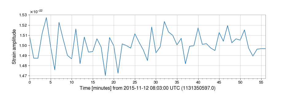
Demodulation is useful when trying to examine steady sinusoidal signals we know to be contained within data. For instance, we can download some data from GWOSC to look at trends of the amplitude and phase of LIGO Livingston’s calibration line at 331.3 Hz:

>>> from gwpy.timeseries import TimeSeries
>>> data = TimeSeries.fetch_open_data('L1', 1131350417, 1131357617)

We can demodulate the TimeSeries at 331.3 Hz with a stride of one minute:

>>> amp, phase = data.demodulate(331.3, stride=60)

We can then plot these trends to visualize fluctuations in the amplitude of the calibration line:

>>> from gwpy.plot import Plot
>>> plot = Plot(amp)
>>> ax = plot.gca()
>>> ax.set_ylabel('Strain Amplitude at 331.3 Hz')
>>> plot.show()

(png)

../../_images/gwpy-timeseries-TimeSeries-2.png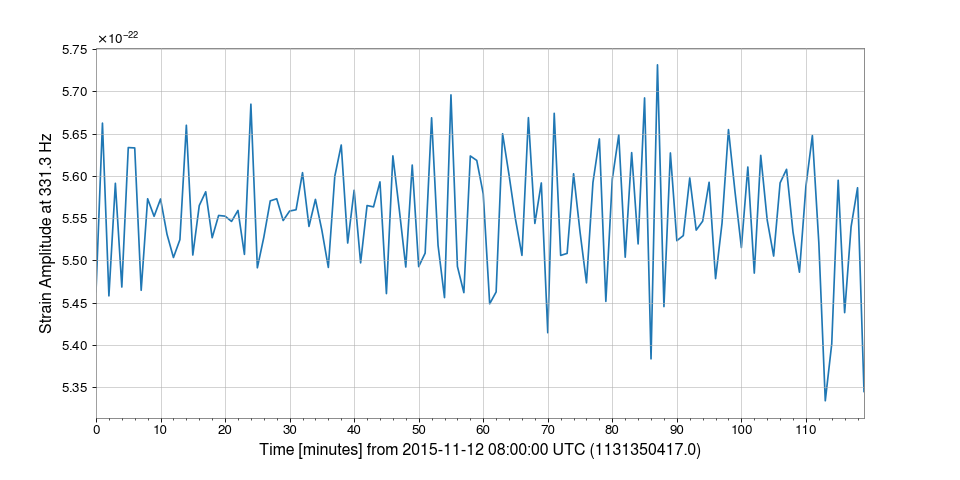

detrend(detrend: Literal['constant', 'linear'] = 'constant') → Self[source]#

Remove the trend from this TimeSeries.

This method just wraps scipy.signal.detrend() to return an object of the same type as the input.

Parameters:

detrendstr, optional: the type of detrending.

Returns:

detrendedTimeSeries: the detrended input series

See also

scipy.signal.detrend: for details on the options for the detrend argument, and how the operation is done

fft(nfft: int | None = None) → FrequencySeries[source]#

Compute the one-dimensional discrete Fourier transform of this TimeSeries.

Parameters:

nfftint, optional: Length of the desired Fourier transform, input will be cropped or padded to match the desired length. If nfft is not given, the length of the TimeSeries will be used.

Returns:

outFrequencySeries: The normalised, complex-valued FFT FrequencySeries.

See also

numpy.fft.rfft: The FFT implementation used in this method.

Notes

This method, in constrast to the numpy.fft.rfft() method it calls, applies the necessary normalisation such that the amplitude of the output FrequencySeries is correct.

fftgram(

fftlength: float,

overlap: float | None = None,

window: WindowLike = 'hann',

**kwargs,

) → Spectrogram[source]#

Calculate the Fourier-gram of this TimeSeries.

At every stride, a single, complex FFT is calculated.

Parameters:

fftlengthfloat: Number of seconds in single FFT.
overlapfloat, optional: Number of seconds of overlap between FFTs, defaults to the recommended overlap for the given window (if given), or 0.
windowstr, numpy.ndarray, optional: Window function to apply to timeseries prior to FFT, see scipy.signal.get_window() for details on acceptable formats.
kwargs: Other keyword arguments are passed to the scipy.signal.spectrogram() method.

Returns:

spectrogramSpectrogram: A Spectrogram containing the complex-valued output of 1D FFTs at every stride in the input TimeSeries, with each column corresponding to a single FFT.

filter(

filt: FilterCompatible,

*,

analog: bool = False,

unit: str = 'rad/s',

normalize_gain: bool = False,

filtfilt: bool = True,

**kwargs,

) → Self[source]#

Filter this TimeSeries with an IIR or FIR filter.

Parameters:

filtnumpy.ndarray or tuple

The filter to be applied. This can be specified in any of the following forms, with the appropriate number of elements in the tuple:

numpy.ndarray - 1D array of FIR filter coefficients.
tuple[numpy.ndarray, numpy.ndarray] - numerator/demoinator polynomials of the transfer function.
numpy.ndarray - 2D array of SOS coefficients.
tuple[numpy.ndarray, numpy.ndarray, float] - zero-pole-gain representation.

filtfiltbool, optional

Filter forward and backwards to preserve phase, default: False.

analogbool, optional

If True, filter coefficients will be converted from Hz to Z-domain digital representation, default: False.

inplacebool, optional

If True, this array will be overwritten with the filtered version, default: False.

unitstr, optional

For analogue ZPK filters, the units in which the zeros and poles are specified. Either 'Hz' or 'rad/s' (default).

normalize_gainbool, optional

Whether to normalize the gain when converting from Hz to rad/s.

False (default): Multiply zeros/poles by -2π but leave gain unchanged. This matches the LIGO GDS ‘f’ plane convention (plane='f' in s2z()).
True: Normalize gain to preserve frequency response magnitude. Gain is scaled by \(|∏p_i/∏z_i| · (2π)^{(n_p - n_z)}\). Use this when your filter was designed with the transfer function \(H(f) = k·∏(f-z_i)/∏(f-p_i)\) in Hz. This matches the LIGO GDS ‘n’ plane convention (plane='n' in s2z()).

Only used for analogue filters in Hz (analog=True, unit="Hz").

kwargs

Other keyword arguments are passed to the filter method.

Returns:

resultTimeSeries: The filtered version of the input TimeSeries.

Raises:

ValueError: If filt arguments cannot be interpreted properly.

See also

scipy.signal.sosfilt: For details on filtering with second-order sections.
scipy.signal.sosfiltfilt: For details on forward-backward filtering with second-order sections
scipy.signal.lfilter: For details on filtering (without SOS).
scipy.signal.filtfilt: For details on forward-backward filtering (without SOS).

Notes

IIR filters are converted into digital cascading second-order sections before being applied to the data.

FIR filters are passed directly to scipy.signal.lfilter() or scipy.signal.filtfilt() without any conversions.

Examples

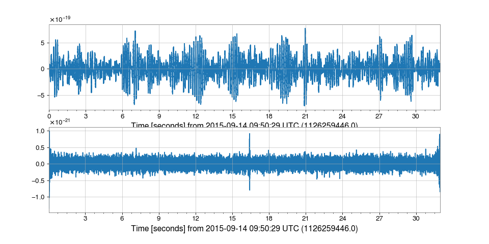
We can design an arbitrarily complicated filter using gwpy.signal.filter_design

>>> from gwpy.signal import filter_design
>>> bp = filter_design.bandpass(50, 250, 4096.)
>>> notches = [filter_design.notch(f, 4096.) for f in (60, 120, 180)]
>>> zpk = filter_design.concatenate_zpks(bp, *notches)

And then can download some data from GWOSC to apply it using TimeSeries.filter:

>>> from gwpy.timeseries import TimeSeries
>>> data = TimeSeries.fetch_open_data('H1', 1126259446, 1126259478)
>>> filtered = data.filter(zpk, filtfilt=True)

We can plot the original signal, and the filtered version, cutting off either end of the filtered data to remove filter-edge artefacts

>>> from gwpy.plot import Plot
>>> plot = Plot(data, filtered[128:-128], separate=True)
>>> plot.show()

(png)

../../_images/gwpy-timeseries-TimeSeries-3.png

find_gates(

tzero: float = 1.0,

*,

whiten: bool = True,

threshold: float = 50.0,

cluster_window: float = 0.5,

**whiten_kwargs,

) → SegmentList[source]#

Identify points that should be gates using a provided threshold.

This method identifies points in the TimeSeries that exceed a provided threshold, and returns a list of segments that should be gated. The gating points are clustered within a provided time window.

This method is useful for identifying high amplitude peaks in the data that should be removed or masked out.

Parameters:

tzeroint, optional: Half-width time duration (seconds) in which the timeseries is set to zero.
whitenbool, optional: If True, data will be whitened before gating points are discovered, use of this option is highly recommended.
thresholdfloat, optional: Amplitude threshold, if the data exceeds this value a gating window will be placed.
cluster_windowfloat, optional: Time duration (seconds) over which gating points will be clustered.
whiten_kwargs: Other keyword arguments will be passed to the TimeSeries.whiten method if it is being used when discovering gating points.

Returns:

outSegmentList: A list of segments that should be gated based on the provided parameters.

See also

TimeSeries.gate: For a method that applies the identified gates.

gate(

tzero: float = 1.0,

tpad: float = 0.5,

*,

whiten: bool = True,

threshold: float = 50.0,

cluster_window: float = 0.5,

**whiten_kwargs,

) → Self[source]#

Remove high amplitude peaks from data using inverse Tukey window.

Points will be discovered automatically using a provided threshold and clustered within a provided time window.

Parameters:

tzeroint, optional: Half-width time duration (seconds) in which the timeseries is set to zero.
tpadint, optional: Half-width time duration (seconds) in which the Tukey window is tapered.
whitenbool, optional: If True, data will be whitened before gating points are discovered, use of this option is highly recommended.
thresholdfloat, optional: Amplitude threshold, if the data exceeds this value a gating window will be placed.
cluster_windowfloat, optional: Time duration (seconds) over which gating points will be clustered.
whiten_kwargs: Other keyword arguments will be passed to the TimeSeries.whiten method if it is being used when discovering gating points.

Returns:

outTimeSeries: A copy of the original TimeSeries that has had gating windows applied.

See also

TimeSeries.mask: For the method that masks out unwanted data.
TimeSeries.find_gates: For the method that identifies gating points.
TimeSeries.whiten: For the whitening filter used to identify gating points.

Examples

Read data into a TimeSeries

>>> from gwpy.timeseries import TimeSeries
>>> data = TimeSeries.fetch_open_data('H1', 1135148571, 1135148771)

Apply gating using custom arguments

>>> gated = data.gate(
...     tzero=1.0,
...     tpad=1.0,
...     threshold=10.0,
...     fftlength=4,
...     overlap=2,
...     method='median',
... )

Plot the original data and the gated data, whiten both for visualization purposes

>>> overlay = data.whiten(4,2,method="median").plot(
...     dpi=150,
...     label="Ungated",
...     color="dodgerblue",
...     zorder=2,
... )
>>> ax = overlay.gca()
>>> ax.plot(
...     gated.whiten(4, 2, method="median"),
...     label="Gated",
...     color="orange",
...     zorder=3,
... )
>>> ax.set_xlim(1135148661, 1135148681)
>>> ax.legend()
>>> overlay.show()

heterodyne( phase: ArrayLike, stride: float = 1, *, singlesided: bool = False, ) → TimeSeries[source]#

Compute the heterodyned average magnitude and phase of this TimeSeries.

Parameters:

phasearray_like: An array of phase measurements (radians) with which to heterodyne the signal.
stridefloat, optional: Stride (seconds) between calculations.
singlesidedbool, optional: Boolean switch to return single-sided output (i.e., to multiply by 2 so that the signal is distributed across positive frequencies only).

Returns:

outTimeSeries: Magnitude and phase trends, represented as mag * exp(1j*phase) with dt=stride.

See also

TimeSeries.demodulate: for a method to heterodyne at a fixed frequency

Notes

This is similar to the demodulate() method, but is more general in that it accepts a varying phase evolution, rather than a fixed frequency.

Unlike demodulate(), the complex output is double-sided by default, so is not multiplied by 2.

Examples

Heterodyning can be useful in analysing quasi-monochromatic signals with a known phase evolution, such as continuous-wave signals from rapidly rotating neutron stars. These sources radiate at a frequency that slowly decreases over time, and is Doppler modulated due to the Earth’s rotational and orbital motion.

To see an example of heterodyning in action, we can simulate a signal whose phase evolution is described by the frequency and its first derivative with respect to time. We can download some O1 era LIGO-Livingston data from GWOSC, inject the simulated signal, and recover its amplitude.

>>> from gwpy.timeseries import TimeSeries
>>> data = TimeSeries.fetch_open_data('L1', 1131350417, 1131354017)

We now need to set the signal parameters, generate the expected phase evolution, and create the signal:

>>> import numpy
>>> f0 = 123.456789  # signal frequency (Hz)
>>> fdot = -9.87654321e-7  # signal frequency derivative (Hz/s)
>>> fepoch = 1131350417  # phase epoch
>>> amp = 1.5e-22  # signal amplitude
>>> phase0 = 0.4  # signal phase at the phase epoch
>>> times = data.times.value - fepoch
>>> phase = 2 * numpy.pi * (f0 * times + 0.5 * fdot * times**2)
>>> signal = TimeSeries(amp * numpy.cos(phase + phase0),
>>>                     sample_rate=data.sample_rate, t0=data.t0)
>>> data = data.inject(signal)

To recover the signal, we can bandpass the injected data around the signal frequency, then heterodyne using our phase model with a stride of 60 seconds:

>>> filtdata = data.bandpass(f0 - 0.5, f0 + 0.5)
>>> het = filtdata.heterodyne(phase, stride=60, singlesided=True)

We can then plot signal amplitude over time (cropping the first two minutes to remove the filter response):

>>> plot = het.crop(het.x0.value + 180).abs().plot()
>>> ax = plot.gca()
>>> ax.set_ylabel("Strain amplitude")
>>> plot.show()

(png)

../../_images/gwpy-timeseries-TimeSeries-4.png

highpass(

frequency: float,

gpass: float = 2,

gstop: float = 30,

fstop: float | None = None,

type: Literal['fir', 'iir'] = 'iir',

*,

filtfilt: bool = True,

**kwargs,

) → TimeSeries[source]#

Filter this TimeSeries with a high-pass filter.

Parameters:

frequencyfloat: High-pass corner frequency.
gpassfloat: The maximum loss in the passband (dB).
gstopfloat: The minimum attenuation in the stopband (dB).
fstopfloat: Stop-band edge frequency, defaults to frequency * 1.5.
typestr: The filter type, either 'iir' or 'fir'.
filtfiltbool, optional: If True, apply the filter using a forward-backward filter design, otherwise apply the filter in a single pass. Defaults to True.
kwargs: Other keyword arguments are passed to gwpy.signal.filter_design.highpass().

Returns:

hpseriesTimeSeries: A high-passed version of the input TimeSeries.

See also

gwpy.signal.filter_design.highpass: For details on the filter design.
TimeSeries.filter: For details on how the filter is applied.

lowpass(

frequency: float,

gpass: float = 2,

gstop: float = 30,

fstop: float | None = None,

type: Literal['fir', 'iir'] = 'iir',

*,

filtfilt: bool = True,

**kwargs,

) → TimeSeries[source]#

Filter this TimeSeries with a Butterworth low-pass filter.

Parameters:

frequencyfloat: Low-pass corner frequency.
gpassfloat: The maximum loss in the passband (dB).
gstopfloat: The minimum attenuation in the stopband (dB).
fstopfloat: Stop-band edge frequency, defaults to frequency * 1.5.
typestr: The filter type, either 'iir' or 'fir'.
filtfiltbool, optional: If True, apply the filter using a forward-backward filter design, otherwise apply the filter in a single pass. Defaults to True.
kwargs: Other keyword arguments are passed to gwpy.signal.filter_design.lowpass().

Returns:

lpseriesTimeSeries: A low-passed version of the input TimeSeries.

See also

gwpy.signal.filter_design.lowpass: For details on the filter design.
TimeSeries.filter: For details on how the filter is applied.

mask(

deadtime: SegmentList | None = None,

flag: str | None = None,

*,

query_open_data: bool = False,

const: float = nan,

tpad: float = 0.5,

inplace: bool = False,

**kwargs,

) → Self[source]#

Mask portions of this TimeSeries that fall within a given list of segments.

Parameters:

deadtimeSegmentList, optional: A list of time segments defining the deadtime (i.e., masked portions) of the output, will supersede flag if given.
flagstr, optional: The name of a data-quality flag for which to query, required if deadtime is not given.
query_open_databool, optional: If True, will query for publicly released data-quality segments through the Gravitational-wave Open Science Center (GWOSC).
constfloat, optional: Constant value with which to mask deadtime data.
tpadfloat, optional: Length of time (in seconds) over which to taper off data at mask segment boundaries.
inplacebool, optional: If True, this array will be overwritten with the masked version, otherwise (False, default) a modified copy will be returned.
kwargsdict, optional: Additional keyword arguments to query or fetch_open_data, see “Notes” below.

Returns:

outTimeSeries: The masked version of this TimeSeries.

See also

gwpy.segments.DataQualityFlag.query: For the method to query segments of a given data-quality flag.
gwpy.segments.DataQualityFlag.fetch_open_data: For the method to query data-quality flags from the GWOSC database.
scipy.signal.windows.tukey: For the Tukey (tapered cosine) window used for tapering.

Notes

If tpad is nonzero, the Tukey (tapered cosine) window is used to smoothly ramp data down to zero over a timescale tpad approaching every segment boundary in deadtime. However, this does not apply to the left or right bounds of the original TimeSeries.

The deadtime segment list will always be coalesced and restricted to the limits of self.span. In particular, when querying a data-quality flag, this means the start and end arguments to query will effectively be reset and therefore need not be given.

If flag is interpreted positively, i.e. if flag being active corresponds to a “good” state, then its complement in self.span will be used to define the deadtime for masking.

notch(

frequency: QuantityLike,

type: Literal['iir'] = 'iir',

*,

filtfilt: bool = True,

**kwargs,

) → Self[source]#

Notch out a frequency in this TimeSeries.

Parameters:

frequencyfloat, Quantity: Frequency (default in Hertz) at which to apply the notch.
typestr, optional: Type of filter to apply, currently only ‘iir’ is supported.
filtfiltbool, optional: Whether to apply zero-phase filtering (default is True).
kwargs: Other keyword arguments to pass to gwpy.signal.filter_design.notch.

Returns:

notchedTimeSeries: A notch-filtered copy of the input TimeSeries.

See also

TimeSeries.filter: For details on the filtering method.
gwpy.signal.filter_design.notch: For details on the IIR filter design method.

psd(

fftlength: float | None = None,

overlap: float | None = None,

window: WindowLike = 'hann',

method: str = 'median',

**kwargs,

) → FrequencySeries[source]#

Calculate the PSD FrequencySeries for this TimeSeries.

Parameters:

fftlengthfloat: Number of seconds in single FFT, defaults to a single FFT covering the full duration.
overlapfloat, optional: Number of seconds of overlap between FFTs, defaults to the recommended overlap for the given window (if given), or 0.
windowstr, numpy.ndarray, optional: Window function to apply to timeseries prior to FFT, see scipy.signal.get_window() for details on acceptable formats.
methodstr, optional: FFT-averaging method (default: 'median'), see Notes for more details.
kwargs: Other keyword arguments are passed to the underlying PSD-generation method.

Returns:

psdFrequencySeries: A data series containing the PSD.

Notes

The accepted method arguments are:

'bartlett' : a mean average of non-overlapping periodograms
'median' : a median average of overlapping periodograms
'welch' : a mean average of overlapping periodograms

q_gram(

qrange: tuple[float, float] = (4, 64),

frange: tuple[float, float] = (0, inf),

mismatch: float = 0.2,

snrthresh: float = 5.5,

**kwargs,

) → EventTable[source]#

Scan a TimeSeries using the multi-Q transform.

Parameters:

qrangetuple of float, optional: (low, high) range of Qs to scan.
frangetuple of float, optional: (low, high) range of frequencies to scan.
mismatchfloat, optional: Maximum allowed fractional mismatch between neighbouring tiles.
snrthreshfloat, optional: Lower inclusive threshold on individual tile SNR to keep in the table.
kwargs: Other keyword arguments to be passed to QTiling.transform(), including 'epoch' and 'search'.

Returns:

qgramEventTable: A table of time-frequency tiles on the most significant QPlane.

See also

TimeSeries.q_transform: For a method to interpolate the raw Q-transform over a regularly gridded spectrogram.
gwpy.signal.qtransform: For code and documentation on how the Q-transform is implemented.
gwpy.table.EventTable.tile: To render this EventTable as a collection of polygons.

Notes

Only tiles with signal energy greater than or equal to snrthresh ** 2 / 2 will be stored in the output EventTable. The table columns are 'time', 'duration', 'frequency', 'bandwidth', and 'energy'.

q_transform(

qrange: tuple[float, float] = (4, 64),

frange: tuple[float, float] = (0, inf),

gps: float | None = None,

search: float = 0.5,

tres: str | float = '<default>',

fres: str | float = '<default>',

*,

logf: bool = False,

norm: str = 'median',

mismatch: float = 0.2,

outseg: Segment | None = None,

whiten: bool | FrequencySeries = True,

fduration: float = 2,

highpass: float | None = None,

**asd_kw,

) → Spectrogram[source]#

Compute the multi-Q transform and return an interpolated spectrogram.

By default, this method returns a high-resolution spectrogram in both time and frequency, which can result in a large memory footprint. If you know that you only need a subset of the output for, say, a figure, consider using outseg and the other keyword arguments to restrict the size of the returned data.

Parameters:

qrangetuple of float, optional: (low, high) range of Qs to scan.
frangetuple of float, optional: (log, high) range of frequencies to scan.
gpsfloat, optional: Central time of interest for determine loudest Q-plane.
searchfloat, optional: Window around gps in which to find peak energies, only used if gps is given.
tresfloat, optional: Desired time resolution (seconds) of output Spectrogram, default is abs(outseg) / 1000.
fresfloat, int, None, optional: Desired frequency resolution (Hertz) of output Spectrogram, or, if logf=True, the number of frequency samples; give None to skip this step and return the original resolution, default is 0.5 Hz or 500 frequency samples.
logfbool, optional: If True, use logarithmically sampled frequencies in the output (using fres as the number of frequency samples), otherwise use linearly sampled frequencies of the specified resolution.
normbool, str, optional: If True normalise the returned Q-transform output by the median; if False do not normalize; if a string, specify how to normalize the output, e.g. 'mean' or 'median'.
mismatchfloat: Maximum allowed fractional mismatch between neighbouring tiles.
outsegSegment, optional: GPS [start, stop) segment for output Spectrogram, default is the full duration of the input.
whitenbool, FrequencySeries, optional: If True, whiten the data before computing the Q-transform; if False, do not whiten the data; if a FrequencySeries, use that as the amplitude spectral density (ASD) to whiten the data.
fdurationfloat, optional: Duration (in seconds) of the time-domain FIR whitening filter, only used if whiten is not False, defaults to 2 seconds.
highpassfloat, optional: Highpass corner frequency (in Hz) of the FIR whitening filter, used only if whiten is not False, default: None.
asd_kw: Keyword arguments to pass to TimeSeries.asd to generate an ASD to use when whitening the data.

Returns:

outSpectrogram: Output Spectrogram of normalised Q energy.

See also

TimeSeries.asd: For documentation on acceptable **asd_kw.
TimeSeries.whiten: For documentation on how the whitening is done.
gwpy.signal.qtransform: For code and documentation on how the Q-transform is implemented.

Notes

This method will return a Spectrogram of dtype float32 if norm is given, and float64 otherwise.

To optimize plot rendering with pcolormesh, the output Spectrogram can be given a log-sampled frequency axis by passing logf=True at runtime. The fres argument is then the number of points on the frequency axis. Note, this is incompatible with imshow.

It is also highly recommended to use the outseg keyword argument when only a small window around a given GPS time is of interest. This will speed up this method a little, but can greatly speed up rendering the resulting Spectrogram using pcolormesh.

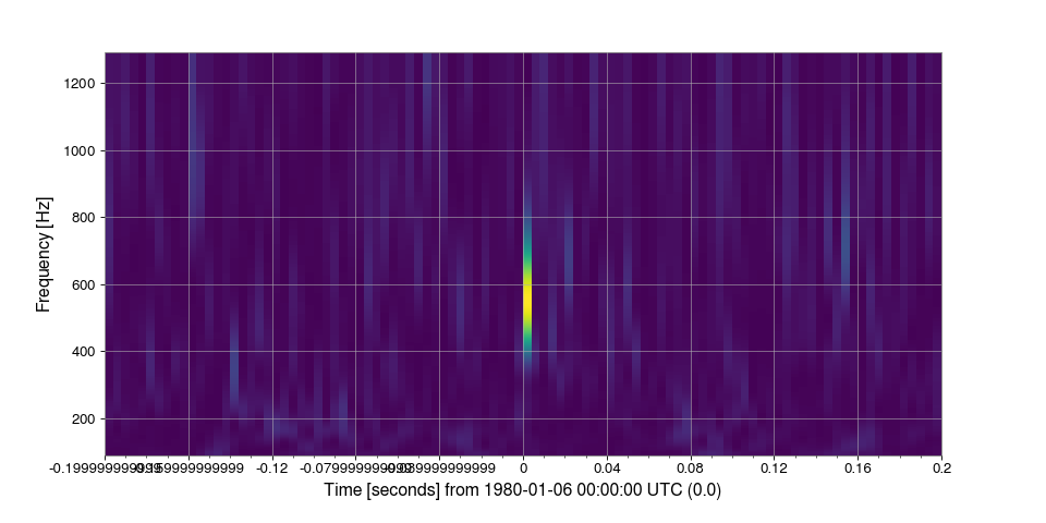
If you aren’t going to use pcolormesh in the end, don’t worry.

Examples

>>> from numpy.random import normal
>>> from scipy.signal import gausspulse
>>> from gwpy.timeseries import TimeSeries

Generate a TimeSeries containing Gaussian noise sampled at 4096 Hz, centred on GPS time 0, with a sine-Gaussian pulse (‘glitch’) at 500 Hz:

>>> noise = TimeSeries(
...     normal(loc=1, size=4096*4),
...     sample_rate=4096,
...     epoch=-2,
... )
>>> glitch = TimeSeries(
...     gausspulse(noise.times.value, fc=500) * 4,
...     sample_rate=4096,
... )
>>> data = noise + glitch

Compute and plot the Q-transform of these data:

>>> q = data.q_transform()
>>> plot = q.plot()
>>> ax = plot.gca()
>>> ax.set_xlim(-.2, .2)
>>> ax.set_epoch(0)
>>> plot.show()

(png)

../../_images/gwpy-timeseries-TimeSeries-5.png

rayleigh_spectrogram(

stride: float,

fftlength: float | None = None,

overlap: float = 0,

window: WindowLike = 'hann',

nproc: int = 1,

**kwargs,

) → Spectrogram[source]#

Calculate the Rayleigh statistic spectrogram of this TimeSeries.

Parameters:

stridefloat: Number of seconds in single PSD (column of spectrogram).
fftlengthfloat: Number of seconds in single FFT.
overlapfloat, optional: Number of seconds of overlap between FFTs, passing None will choose based on the window method, default: 0.
windowstr, numpy.ndarray, optional: Window function to apply to timeseries prior to FFT, see scipy.signal.get_window() for details on acceptable formats.
nprocint, optional: Maximum number of independent frame reading processes, default is set to single-process file reading.
kwargs: Other keyword arguments are passed to the underlying Rayleigh statistic calculation.

Returns:

spectrogramSpectrogram: Time-frequency Rayleigh spectrogram as generated from the input time-series.

See also

TimeSeries.rayleigh: For details of the statistic calculation.

rayleigh_spectrum( fftlength: float | None = None, overlap: float = 0, window: WindowLike = 'hann', ) → FrequencySeries[source]#

Calculate the Rayleigh FrequencySeries for this TimeSeries.

The Rayleigh statistic is calculated as the ratio of the standard deviation and the mean of a number of periodograms.

Parameters:

fftlengthfloat: Number of seconds in single FFT, defaults to a single FFT covering the full duration.
overlapfloat, optional: Number of seconds of overlap between FFTs, passing None will choose based on the window method, default: 0.
windowstr, numpy.ndarray, optional: Window function to apply to timeseries prior to FFT, see scipy.signal.get_window() for details on acceptable formats.

Returns:

psdFrequencySeries: A data series containing the PSD.

resample( rate: float, window: WindowLike = 'hamming', ftype: Literal['fir', 'iir'] = 'fir', n: int | None = None, ) → TimeSeries[source]#

Resample this Series to a new rate.

Upsampling, or downsampling by a non-integer factor calls out to scipy.signal.resample(), while integer downsampling calls out to scipy.signal.decimate().

Parameters:

ratefloat, astropy.units.Quantity: Rate to which to resample this Series.
windowstr, numpy.ndarray, optional: Window function to apply to signal in the Fourier domain, see scipy.signal.get_window() for details on acceptable formats, only used for ftype='fir' or irregular downsampling.
ftypestr, optional: Type of filter, either ‘fir’ or ‘iir’, defaults to ‘fir’.
nint, optional: If ftype='fir' the number of taps in the filter, otherwise the order of the Chebyshev type I IIR filter.

Returns:

Series: A new Series with the resampling applied, and the same metadata.

rms(stride: float = 1) → TimeSeries[source]#

Calculate the root-mean-square value of this TimeSeries once per stride.

Parameters:

stridefloat: stride (seconds) between RMS calculations

Returns:

rmsTimeSeries: a new TimeSeries containing the RMS value with dt=stride

spectral_variance( stride: float, fftlength: float | None = None, overlap: float | None = None, method: str = 'median', window: WindowLike = 'hann', *, nproc: int = 1, filter_: FilterCompatible | None = None, bins: ArrayLike | None = None, low: float | None = None, high: float | None = None, nbins: int = 500, log: bool = False, norm: bool = False, density: bool = False, ) → SpectralVariance[source]#

Calculate the SpectralVariance of this TimeSeries.

Parameters:

stridefloat: Number of seconds in single PSD (column of spectrogram).
fftlengthfloat: Number of seconds in single FFT.
methodstr, optional: FFT-averaging method (default: 'median'), see Notes for more details.
overlapfloat, optional: Number of seconds of overlap between FFTs, defaults to the recommended overlap for the given window (if given), or 0.
windowstr, numpy.ndarray, optional: Window function to apply to timeseries prior to FFT, see scipy.signal.get_window() for details on acceptable formats.
nprocint: Maximum number of independent frame reading processes, default is set to single-process file reading.
filter_FilterCompatible, optional: Filter to apply to each time-bin of the spectrogram prior to variance calculation.
binsnumpy.ndarray, optional, default None: Array of histogram bin edges, including the rightmost edge.
lowfloat, optional: Left edge of lowest amplitude bin, only read if bins is not given.
highfloat, optional: Right edge of highest amplitude bin, only read if bins is not given.
nbinsint, optional: Number of bins to generate, only read if bins is not given.
logbool, optional: Calculate amplitude bins over a logarithmic scale, only read if bins is not given.
normbool, optional: Normalise bin counts to a unit sum.
densitybool, optional: Normalise bin counts to a unit integral.

Returns:

specvarSpectralVariance: 2D-array of spectral frequency-amplitude counts.

See also

numpy.histogram: For details on specifying bins and weights.

Notes

The accepted method arguments are:

'bartlett' : a mean average of non-overlapping periodograms
'median' : a median average of overlapping periodograms
'welch' : a mean average of overlapping periodograms

spectrogram(

stride: float,

fftlength: float | None = None,

overlap: float | None = None,

window: WindowLike = 'hann',

method: str = 'median',

nproc: int = 1,

**kwargs,

) → Spectrogram[source]#

Calculate the average power spectrogram of this TimeSeries.

Each time-bin of the output Spectrogram is calculated by taking a chunk of the TimeSeries in the segment [t - overlap/2., t + stride + overlap/2.) and calculating the psd() of those data.

As a result, each time-bin is calculated using stride + overlap seconds of data.

Parameters:

stridefloat: Number of seconds in single PSD (column of spectrogram).
fftlengthfloat: Number of seconds in single FFT.
overlapfloat, optional: Number of seconds of overlap between FFTs, defaults to the recommended overlap for the given window (if given), or 0.
windowstr, numpy.ndarray, optional: Window function to apply to timeseries prior to FFT, see scipy.signal.get_window() for details on acceptable formats.
methodstr, optional: FFT-averaging method (default: 'median'), see Notes for more details.
nprocint: Number of CPUs to use in parallel processing of FFTs.
kwargs: Other keyword arguments are passed to the underlying PSD-generation method.

Returns:

spectrogramSpectrogram: Time-frequency power spectrogram as generated from the input time-series.

Notes

The accepted method arguments are:

'bartlett' : a mean average of non-overlapping periodograms
'median' : a median average of overlapping periodograms
'welch' : a mean average of overlapping periodograms

spectrogram2(

fftlength: float,

overlap: float | None = None,

window: WindowLike = 'hann',

**kwargs,

) → Spectrogram[source]#

Calculate the non-averaged power Spectrogram of this TimeSeries.

Parameters:

fftlengthfloat: Number of seconds in single FFT.
overlapfloat, optional: Number of seconds of overlap between FFTs, defaults to the recommended overlap for the given window (if given), or 0
windowstr, numpy.ndarray, optional: Window function to apply to timeseries prior to FFT, see scipy.signal.get_window() for details on acceptable formats.
scaling[ ‘density’ | ‘spectrum’ ], optional: Selects between computing the power spectral density (‘density’) where the Spectrogram has units of V**2/Hz if the input is measured in V and computing the power spectrum (‘spectrum’) where the Spectrogram has units of V**2 if the input is measured in V. Defaults to ‘density’.
kwargs: Other parameters to be passed to scipy.signal.periodogram for each column of the Spectrogram.

Returns:

spectrogram: Spectrogram: A power Spectrogram with 1/fftlength frequency resolution and (fftlength - overlap) time resolution.

See also

scipy.signal.periodogram: For documentation on the Fourier methods used in this calculation.

Notes

This method calculates overlapping periodograms for all possible chunks of data entirely containing within the span of the input TimeSeries, then normalises the power in overlapping chunks using a triangular window centred on that chunk which most overlaps the given Spectrogram time sample.

taper( side: Literal['left', 'right', 'leftright'] = 'leftright', duration: float | None = None, nsamples: int | None = None, ) → Self[source]#

Taper the ends of this TimeSeries smoothly to zero.

Parameters:

sidestr, optional: The side of the TimeSeries to taper, must be one of 'left', 'right', or 'leftright'.
durationfloat, optional: The duration of time to taper, will override nsamples if both are provided as arguments.
nsamplesint, optional: The number of samples to taper, will be overridden by duration if both are provided as arguments.

Returns:

outTimeSeries: A copy of self tapered at one or both ends.

Raises:

ValueError: If side is not one of ('left', 'right', 'leftright').

Notes

The TimeSeries.taper() automatically tapers from the second stationary point (local maximum or minimum) on the specified side of the input. However, the method will never taper more than half the full width of the TimeSeries, and will fail if there are no stationary points.

See scipy.signal.windows.tukey() for the Tukey (tapered cosine) window used for tapering, and see scipy.signal.get_window() for other common window formats.

Examples

To see the effect of the Tukey (tapered cosine) window, we can taper a sinusoidal TimeSeries at both ends:

>>> import numpy
>>> from gwpy.timeseries import TimeSeries
>>> t = numpy.linspace(0, 1, 2048)
>>> series = TimeSeries(numpy.cos(10.5*numpy.pi*t), times=t)
>>> tapered = series.taper()

We can plot it to see how the ends now vary smoothly from 0 to 1:

>>> from gwpy.plot import Plot
>>> plot = Plot(series, tapered, separate=True, sharex=True)
>>> plot.show()

(png)

../../_images/gwpy-timeseries-TimeSeries-6.png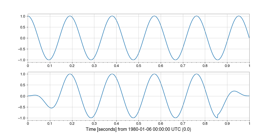

transfer_function(

other: TimeSeries,

fftlength: float | None = None,

overlap: float | None = None,

window: WindowLike = 'hann',

average: str = 'mean',

**kwargs,

) → FrequencySeries[source]#

Calculate the transfer function between this TimeSeries and another.

This TimeSeries is the ‘A-channel’, serving as the reference (denominator) while the other time series is the test (numerator)

Parameters:

otherTimeSeries: TimeSeries signal to calculate the transfer function with.
fftlengthfloat, optional: Number of seconds in single FFT, defaults to a single FFT covering the full duration.
overlapfloat, optional: Number of seconds of overlap between FFTs, defaults to the recommended overlap for the given window (if given), or 0.
windowstr, numpy.ndarray, optional: Window function to apply to timeseries prior to FFT, see scipy.signal.get_window() for details on acceptable formats.
averagestr, optional: FFT-averaging method (default: 'mean') passed to underlying csd() and psd() methods.
kwargs: Any other keyword arguments accepted by TimeSeries.csd() or TimeSeries.psd().

Returns:

transfer_functionFrequencySeries: The transfer function FrequencySeries of this TimeSeries with the other.

Notes

If self and other have difference TimeSeries.sample_rate values, the higher sampled TimeSeries will be down-sampled to match the lower.

whiten(

fftlength: float | None = None,

overlap: float = 0,

method: str = 'median',

window: WindowLike = 'hann',

detrend: Literal['linear', 'constant'] = 'constant',

asd: FrequencySeries | None = None,

fduration: float = 2,

highpass: float | None = None,

**kwargs,

) → Self[source]#

Whiten this TimeSeries using inverse spectrum truncation.

Parameters:

fftlengthfloat, optional: FFT integration length (in seconds) for ASD estimation.
overlapfloat, optional: Number of seconds of overlap between FFTs, defaults to the recommended overlap for the given window (if given), or 0.
methodstr, optional: FFT-averaging method (default: 'median').
windowstr, numpy.ndarray, optional: Window function to apply to timeseries prior to FFT, see scipy.signal.get_window() for details on acceptable formats.
detrendstr, optional: Type of detrending to do before FFT (see detrend for more details).
asdFrequencySeries, optional: The amplitude spectral density using which to whiten the data, overrides other ASD arguments, default: None.
fdurationfloat, optional: Duration (in seconds) of the time-domain FIR whitening filter, must be no longer than fftlength, default: 2 seconds.
highpassfloat, optional: Highpass corner frequency (in Hz) of the FIR whitening filter.
kwargs: Other keyword arguments are passed to the TimeSeries.asd method to estimate the amplitude spectral density FrequencySeries of this TimeSeries.

Returns:

outTimeSeries: A whitened version of the input data with zero mean and unit variance.

See also

TimeSeries.asd: For details on the ASD calculation.
TimeSeries.convolve: For details on convolution with the overlap-save method.
gwpy.signal.filter_design.fir_from_transfer: For FIR filter design through spectrum truncation.

Notes

The accepted method arguments are:

'bartlett' : a mean average of non-overlapping periodograms
'median' : a median average of overlapping periodograms
'welch' : a mean average of overlapping periodograms

The window argument is used in ASD estimation, FIR filter design, and in preventing spectral leakage in the output.

Due to filter settle-in, a segment of length 0.5*fduration will be corrupted at the beginning and end of the output. See convolve for more details.

The input is detrended and the output normalised such that, if the input is stationary and Gaussian, then the output will have zero mean and unit variance.

For more on inverse spectrum truncation, see arXiv:gr-qc/0509116.

zpk(

zeros: ArrayLike1D,

poles: ArrayLike1D,

gain: float,

*,

analog: bool = False,

unit: str = 'rad/s',

normalize_gain: bool = False,

filtfilt: bool = True,

**kwargs,

) → TimeSeries[source]#

Filter this TimeSeries by applying a digital zero-pole-gain filter.

Parameters:

zerosarray-like

Zeros of the transfer function.

polesarray-like

Poles of the transfer function.

gainfloat

System gain.

analogbool, optional

Type of filter being applied. If analog=True the zeros/poles/gain will be transformed from analogue (s-plane) to digital (z-plane) representation using the bilinear transform.

unitstr

For analogue ZPK filters, the units in which the zeros and poles are specified. Either 'Hz' or 'rad/s' (default).

normalize_gainbool, optional

Whether to normalize the gain when converting from Hz to rad/s.

False (default): Multiply zeros/poles by -2π but leave gain unchanged. This matches the LIGO GDS ‘f’ plane convention (plane='f' in s2z()).
True: Normalize gain to preserve frequency response magnitude. Gain is scaled by \(|∏p_i/∏z_i| · (2π)^{(n_p - n_z)}\). Use this when your filter was designed with the transfer function \(H(f) = k·∏(f-z_i)/∏(f-p_i)\) in Hz. This matches the LIGO GDS ‘n’ plane convention (plane='n' in s2z()).

Only used for analogue filters in Hz (analog=True, unit="Hz").

filtfiltbool, optional

If True (default), apply the filter using a forward-backward filter design, otherwise apply the filter in a single pass.

kwargs

Other keyword arguments are passed to the filter method.

Returns:

timeseriesTimeSeries: The filtered version of the input data.

See also

TimeSeries.filter: For details on how a digital ZPK-format filter is applied.
gwpy.signal.filter_design.prepare_digital_filter: For details on preparing the digital ZPK filter for application.

Examples

To apply a zpk filter with file poles at 100 Hz, and five zeros at 1 Hz (giving an overall DC gain of 1e-10):

>>> data2 = data.zpk([100]*5, [1]*5, 1e-10)