Axes#
- class gwpy.plot.Axes( )[source]#
Bases:
AxesGWpy customised
Axes.Methods Summary
colorbar([mappable, fraction])draw(renderer)Draw the Artist (and its children) using the given renderer.
Return the epoch for the current GPS scale/.
hist(x[, bins])Compute and plot a histogram.
imshow(X[, cmap, norm])Display an image, i.e. data on a 2D regular raster.
legend(*args, **kwargs)Place a legend on the Axes.
pcolormesh(*args, **kwargs)Create a pseudocolor plot with a non-regular rectangular grid.
plot_mmm(data[, lower, upper])Plot a
Seriesas a line, with a shaded region around it.scatter(x, y[, s, c])A scatter plot of y vs. x with varying marker size and/or color.
set(*[, adjustable, agg_filter, alpha, ...])Set multiple properties at once.
set_epoch(epoch)Set the epoch for the current GPS scale.
set_xlim([left, right, emit, auto, xmin, xmax])Set the x-axis view limits.
tile(x, y, w, h[, color, anchor, ...])Plot rectanguler tiles based onto these
Axes.Methods Documentation
- colorbar( ) Colorbar[source]#
-
- Parameters:
- mappable
matplotlibdatacollection, optional Collection against which to map the colouring, default will be the last added mappable artist (collection or image).
- fraction
float, optional Fraction of space to steal from these
Axesto make space for the new axes, default is0.. Usefraction=.15to match the upstream matplotlib default.- **kwargs
other keyword arguments to be passed to the
Plot.colorbar()generator
- mappable
- Returns:
- cbar
Colorbar the newly added
Colorbar
- cbar
See also
- draw(renderer)#
Draw the Artist (and its children) using the given renderer.
This has no effect if the artist is not visible (
Artist.get_visiblereturns False).- Parameters:
- renderer
RendererBasesubclass.
- renderer
Notes
This method is overridden in the Artist subclasses.
- get_epoch() float | None[source]#
Return the epoch for the current GPS scale/.
This method will fail if the current X-axis scale isn’t one of the GPS scales. See Plotting GPS time scales for more details.
- hist( ) tuple[numpy.ndarray | list[numpy.ndarray], numpy.ndarray, BarContainer | Polygon | list[BarContainer | Polygon]][source]#
Compute and plot a histogram.
This method uses
numpy.histogramto bin the data in x and count the number of values in each bin, then draws the distribution either as aBarContainerorPolygon. The bins, range, density, and weights parameters are forwarded tonumpy.histogram.If the data has already been binned and counted, use
barorstairsto plot the distribution:counts, bins = np.histogram(x) plt.stairs(counts, bins)
Alternatively, plot pre-computed bins and counts using
hist()by treating each bin as a single point with a weight equal to its count:plt.hist(bins[:-1], bins, weights=counts)
The data input x can be a singular array, a list of datasets of potentially different lengths ([x0, x1, …]), or a 2D ndarray in which each column is a dataset. Note that the ndarray form is transposed relative to the list form. If the input is an array, then the return value is a tuple (n, bins, patches); if the input is a sequence of arrays, then the return value is a tuple ([n0, n1, …], bins, [patches0, patches1, …]).
Masked arrays are not supported.
- Parameters:
- x(n,)
arrayor sequence of (n,)arrays Input values, this takes either a single array or a sequence of arrays which are not required to be of the same length.
- bins
intor sequence orstr, default:rcParams[“hist.bins”](default:10) If bins is an integer, it defines the number of equal-width bins in the range.
If bins is a sequence, it defines the bin edges, including the left edge of the first bin and the right edge of the last bin; in this case, bins may be unequally spaced. All but the last (righthand-most) bin is half-open. In other words, if bins is:
[1, 2, 3, 4]
then the first bin is
[1, 2)(including 1, but excluding 2) and the second[2, 3). The last bin, however, is[3, 4], which includes 4.If bins is a string, it is one of the binning strategies supported by
numpy.histogram_bin_edges: ‘auto’, ‘fd’, ‘doane’, ‘scott’, ‘stone’, ‘rice’, ‘sturges’, or ‘sqrt’.- range
tupleorNone, default:None The lower and upper range of the bins. Lower and upper outliers are ignored. If not provided, range is
(x.min(), x.max()). Range has no effect if bins is a sequence.If bins is a sequence or range is specified, autoscaling is based on the specified bin range instead of the range of x.
- densitybool, default:
False If
True, draw and return a probability density: each bin will display the bin’s raw count divided by the total number of counts and the bin width (density = counts / (sum(counts) * np.diff(bins))), so that the area under the histogram integrates to 1 (np.sum(density * np.diff(bins)) == 1).If stacked is also
True, the sum of the histograms is normalized to 1.- weights(n,) array_like or
None, default:None An array of weights, of the same shape as x. Each value in x only contributes its associated weight towards the bin count (instead of 1). If density is
True, the weights are normalized, so that the integral of the density over the range remains 1.- cumulativebool or -1, default:
False If
True, then a histogram is computed where each bin gives the counts in that bin plus all bins for smaller values. The last bin gives the total number of datapoints.If density is also
Truethen the histogram is normalized such that the last bin equals 1.If cumulative is a number less than 0 (e.g., -1), the direction of accumulation is reversed. In this case, if density is also
True, then the histogram is normalized such that the first bin equals 1.- bottomarray_like or
float, default: 0 Location of the bottom of each bin, i.e. bins are drawn from
bottomtobottom + hist(x, bins)If a scalar, the bottom of each bin is shifted by the same amount. If an array, each bin is shifted independently and the length of bottom must match the number of bins. If None, defaults to 0.- histtype{‘bar’, ‘barstacked’, ‘step’, ‘stepfilled’}, default: ‘bar’
The type of histogram to draw.
‘bar’ is a traditional bar-type histogram. If multiple data are given the bars are arranged side by side.
‘barstacked’ is a bar-type histogram where multiple data are stacked on top of each other.
‘step’ generates a lineplot that is by default unfilled.
‘stepfilled’ generates a lineplot that is by default filled.
- align{‘left’, ‘mid’, ‘right’}, default: ‘mid’
The horizontal alignment of the histogram bars.
‘left’: bars are centered on the left bin edges.
‘mid’: bars are centered between the bin edges.
‘right’: bars are centered on the right bin edges.
- orientation{‘vertical’, ‘horizontal’}, default: ‘vertical’
If ‘horizontal’,
barhwill be used for bar-type histograms and the bottom kwarg will be the left edges.- rwidth
floatorNone, default:None The relative width of the bars as a fraction of the bin width. If
None, automatically compute the width.Ignored if histtype is ‘step’ or ‘stepfilled’.
- logbool, default:
False If
True, the histogram axis will be set to a log scale.- logbinsbool, optional
If
True, use logarithmically-spaced histogram bins.Default is
False- colorcolor or
listof color orNone, default:None Color or sequence of colors, one per dataset. Default (
None) uses the standard line color sequence.- label
strorlistofstr, optional String, or sequence of strings to match multiple datasets. Bar charts yield multiple patches per dataset, but only the first gets the label, so that
legendwill work as expected.- stackedbool, default:
False If
True, multiple data are stacked on top of each other IfFalsemultiple data are arranged side by side if histtype is ‘bar’ or on top of each other if histtype is ‘step’
- x(n,)
- Returns:
- n
arrayorlistofarrays The values of the histogram bins. See density and weights for a description of the possible semantics. If input x is an array, then this is an array of length nbins. If input is a sequence of arrays
[data1, data2, ...], then this is a list of arrays with the values of the histograms for each of the arrays in the same order. The dtype of the array n (or of its element arrays) will always be float even if no weighting or normalization is used.- bins
array The edges of the bins. Length nbins + 1 (nbins left edges and right edge of last bin). Always a single array even when multiple data sets are passed in.
- patches
BarContainerorlistofasinglePolygonorlistofsuchobjects Container of individual artists used to create the histogram or list of such containers if there are multiple input datasets.
- n
- Other Parameters:
- data
indexableobject, optional If given, the following parameters also accept a string
s, which is interpreted asdata[s]ifsis a key indata:x, weights
- **kwargs
Patchproperties. The following properties additionally accept a sequence of values corresponding to the datasets in x: edgecolor, facecolor, linewidth, linestyle, hatch.Added in version 3.10: Allowing sequences of values in above listed Patch properties.
- data
See also
hist2d2D histogram with rectangular bins
hexbin2D histogram with hexagonal bins
stairsPlot a pre-computed histogram
barPlot a pre-computed histogram
Notes
For large numbers of bins (>1000), plotting can be significantly accelerated by using
stairsto plot a pre-computed histogram (plt.stairs(*np.histogram(data))), or by setting histtype to ‘step’ or ‘stepfilled’ rather than ‘bar’ or ‘barstacked’.
- imshow(
- X: ArrayLike | PIL.Image.Image,
- cmap: str | Colormap | None = None,
- norm: str | Normalize | None = None,
- **kwargs,
Display an image, i.e. data on a 2D regular raster.
If
arrayis aArray2D(e.g. aSpectrogram), then the defaults are _different_ to those in the upstreamimshow()method. Namely, the defaults areorigin='lower'(coordinates start in lower-left corner)aspect='auto'(pixels are not forced to be square)interpolation='none'(no image interpolation is used)
In all other usage, the defaults from the upstream matplotlib method are unchanged.
- Parameters:
- Xarray_like or
PILimage The image data.
- cmap
strorColormap, default:rcParams[“image.cmap”](default:'viridis') The Colormap instance or registered colormap name used to map scalar data to colors.
- norm
strorNormalize, optional The normalization method used to scale scalar data to the [0, 1] range before mapping to colors using cmap. By default, a linear scaling is used, mapping the lowest value to 0 and the highest to 1.
If given, this can be one of the following:
An instance of
Normalizeor one of its subclasses (see Colormap normalization).A scale name, i.e. one of “linear”, “log”, “symlog”, “logit”, etc. For a list of available scales, call
matplotlib.scale.get_scale_names(). In that case, a suitableNormalizesubclass is dynamically generated and instantiated.
- *args, **kwargs
All arguments and keywords are passed to the inherited
imshow()method.
- Xarray_like or
See also
matplotlib.axes.Axes.imshowfor details of the image rendering
- legend(*args, **kwargs) Legend[source]#
Place a legend on the Axes.
Note
This method uses a custom default legend handler for
Line2Dobjects, with increased linewidth relative to the upstreamlegend()method. To disable this, passhandler_map=None, or create and pass your own handler class. See Custom legends in GWpy for more details.Call signatures:
legend()
legend(handles, labels)
legend(handles=handles)
legend(labels)
The call signatures correspond to the following different ways to use this method:
1. Automatic detection of elements to be shown in the legend
The elements to be added to the legend are automatically determined, when you do not pass in any extra arguments.
In this case, the labels are taken from the artist. You can specify them either at artist creation or by calling the
set_label()method on the artist:ax.plot([1, 2, 3], label='Inline label') ax.legend()
or:
line, = ax.plot([1, 2, 3])
line.set_label('Label via method')
ax.legend()
Note
Specific artists can be excluded from the automatic legend element selection by using a label starting with an underscore, “_”. A string starting with an underscore is the default label for all artists, so calling
Axes.legendwithout any arguments and without setting the labels manually will result in aUserWarningand an empty legend being drawn.2. Explicitly listing the artists and labels in the legend
For full control of which artists have a legend entry, it is possible to pass an iterable of legend artists followed by an iterable of legend labels respectively:
ax.legend([line1, line2, line3], ['label1', 'label2', 'label3'])
3. Explicitly listing the artists in the legend
This is similar to 2, but the labels are taken from the artists’ label properties. Example:
line1, = ax.plot([1, 2, 3], label='label1')
line2, = ax.plot([1, 2, 3], label='label2')
ax.legend(handles=[line1, line2])
4. Labeling existing plot elements
Discouraged
This call signature is discouraged, because the relation between plot elements and labels is only implicit by their order and can easily be mixed up.
To make a legend for all artists on an Axes, call this function with an iterable of strings, one for each legend item. For example:
ax.plot([1, 2, 3])
ax.plot([5, 6, 7])
ax.legend(['First line', 'Second line'])
- Parameters:
- handles
listof (ArtistortupleofArtist), optional A list of Artists (lines, patches) to be added to the legend. Use this together with labels, if you need full control on what is shown in the legend and the automatic mechanism described above is not sufficient.
The length of handles and labels should be the same in this case. If they are not, they are truncated to the smaller length.
If an entry contains a tuple, then the legend handler for all Artists in the tuple will be placed alongside a single label.
- labels
listofstr, optional A list of labels to show next to the artists. Use this together with handles, if you need full control on what is shown in the legend and the automatic mechanism described above is not sufficient.
- handles
- Returns:
- Other Parameters:
- loc
strorpairoffloats, default:rcParams[“legend.loc”](default:'best') The location of the legend.
The strings
'upper left','upper right','lower left','lower right'place the legend at the corresponding corner of the axes.The strings
'upper center','lower center','center left','center right'place the legend at the center of the corresponding edge of the axes.The string
'center'places the legend at the center of the axes.The string
'best'places the legend at the location, among the nine locations defined so far, with the minimum overlap with other drawn artists. This option can be quite slow for plots with large amounts of data; your plotting speed may benefit from providing a specific location.The location can also be a 2-tuple giving the coordinates of the lower-left corner of the legend in axes coordinates (in which case bbox_to_anchor will be ignored).
For back-compatibility,
'center right'(but no other location) can also be spelled'right', and each “string” location can also be given as a numeric value:Location String
Location Code
‘best’ (Axes only)
0
‘upper right’
1
‘upper left’
2
‘lower left’
3
‘lower right’
4
‘right’
5
‘center left’
6
‘center right’
7
‘lower center’
8
‘upper center’
9
‘center’
10
- bbox_to_anchor
BboxBase, 2-tuple, or 4-tuple offloats Box that is used to position the legend in conjunction with loc. Defaults to
axes.bbox(if called as a method toAxes.legend) orfigure.bbox(iffigure.legend). This argument allows arbitrary placement of the legend.Bbox coordinates are interpreted in the coordinate system given by bbox_transform, with the default transform Axes or Figure coordinates, depending on which
legendis called.If a 4-tuple or
BboxBaseis given, then it specifies the bbox(x, y, width, height)that the legend is placed in. To put the legend in the best location in the bottom right quadrant of the Axes (or figure):loc='best', bbox_to_anchor=(0.5, 0., 0.5, 0.5)
A 2-tuple
(x, y)places the corner of the legend specified by loc at x, y. For example, to put the legend’s upper right-hand corner in the center of the Axes (or figure) the following keywords can be used:loc='upper right', bbox_to_anchor=(0.5, 0.5)
- ncols
int, default: 1 The number of columns that the legend has.
For backward compatibility, the spelling ncol is also supported but it is discouraged. If both are given, ncols takes precedence.
- prop
NoneorFontPropertiesordict The font properties of the legend. If None (default), the current
matplotlib.rcParamswill be used.- fontsize
intor {‘xx-small’, ‘x-small’, ‘small’, ‘medium’, ‘large’, ‘x-large’, ‘xx-large’} The font size of the legend. If the value is numeric the size will be the absolute font size in points. String values are relative to the current default font size. This argument is only used if prop is not specified.
- labelcolor
strorlist, default:rcParams[“legend.labelcolor”](default:'None') The color of the text in the legend. Either a valid color string (for example, ‘red’), or a list of color strings. The labelcolor can also be made to match the color of the line or marker using ‘linecolor’, ‘markerfacecolor’ (or ‘mfc’), or ‘markeredgecolor’ (or ‘mec’).
Labelcolor can be set globally using
rcParams[“legend.labelcolor”](default:'None'). If None, usercParams[“text.color”](default:'black').- numpoints
int, default:rcParams[“legend.numpoints”](default:1) The number of marker points in the legend when creating a legend entry for a
Line2D(line).- scatterpoints
int, default:rcParams[“legend.scatterpoints”](default:1) The number of marker points in the legend when creating a legend entry for a
PathCollection(scatter plot).- scatteryoffsetsiterable of
floats, default:[0.375, 0.5, 0.3125] The vertical offset (relative to the font size) for the markers created for a scatter plot legend entry. 0.0 is at the base the legend text, and 1.0 is at the top. To draw all markers at the same height, set to
[0.5].- markerscale
float, default:rcParams[“legend.markerscale”](default:1.0) The relative size of legend markers compared to the originally drawn ones.
- markerfirstbool, default:
True If True, legend marker is placed to the left of the legend label. If False, legend marker is placed to the right of the legend label.
- reversebool, default:
False If True, the legend labels are displayed in reverse order from the input. If False, the legend labels are displayed in the same order as the input.
Added in version 3.7.
- frameonbool, default:
rcParams[“legend.frameon”](default:True) Whether the legend should be drawn on a patch (frame).
- fancyboxbool, default:
rcParams[“legend.fancybox”](default:True) Whether round edges should be enabled around the
FancyBboxPatchwhich makes up the legend’s background.- shadow
None, bool ordict, default:rcParams[“legend.shadow”](default:False) Whether to draw a shadow behind the legend. The shadow can be configured using
Patchkeywords. Customization viarcParams[“legend.shadow”](default:False) is currently not supported.- framealpha
float, default:rcParams[“legend.framealpha”](default:0.8) The alpha transparency of the legend’s background. If shadow is activated and framealpha is
None, the default value is ignored.- facecolor“inherit” or
color, default:rcParams[“legend.facecolor”](default:'inherit') The legend’s background color. If
"inherit", usercParams[“axes.facecolor”](default:'white').- edgecolor“inherit” or
color, default:rcParams[“legend.edgecolor”](default:'0.8') The legend’s background patch edge color. If
"inherit", usercParams[“axes.edgecolor”](default:'black').- mode{“expand”,
None} If mode is set to
"expand"the legend will be horizontally expanded to fill the Axes area (or bbox_to_anchor if defines the legend’s size).- bbox_transform
NoneorTransform The transform for the bounding box (bbox_to_anchor). For a value of
None(default) the Axes’transAxestransform will be used.- title
strorNone The legend’s title. Default is no title (
None).- title_fontproperties
NoneorFontPropertiesordict The font properties of the legend’s title. If None (default), the title_fontsize argument will be used if present; if title_fontsize is also None, the current
rcParams[“legend.title_fontsize”](default:None) will be used.- title_fontsize
intor {‘xx-small’, ‘x-small’, ‘small’, ‘medium’, ‘large’, ‘x-large’, ‘xx-large’}, default:rcParams[“legend.title_fontsize”](default:None) The font size of the legend’s title. Note: This cannot be combined with title_fontproperties. If you want to set the fontsize alongside other font properties, use the size parameter in title_fontproperties.
- alignment{‘center’, ‘left’, ‘right’}, default: ‘center’
The alignment of the legend title and the box of entries. The entries are aligned as a single block, so that markers always lined up.
- borderpad
float, default:rcParams[“legend.borderpad”](default:0.4) The fractional whitespace inside the legend border, in font-size units.
- labelspacing
float, default:rcParams[“legend.labelspacing”](default:0.5) The vertical space between the legend entries, in font-size units.
- handlelength
float, default:rcParams[“legend.handlelength”](default:2.0) The length of the legend handles, in font-size units.
- handleheight
float, default:rcParams[“legend.handleheight”](default:0.7) The height of the legend handles, in font-size units.
- handletextpad
float, default:rcParams[“legend.handletextpad”](default:0.8) The pad between the legend handle and text, in font-size units.
- borderaxespad
float, default:rcParams[“legend.borderaxespad”](default:0.5) The pad between the Axes and legend border, in font-size units.
- columnspacing
float, default:rcParams[“legend.columnspacing”](default:2.0) The spacing between columns, in font-size units.
- handler_map
dictorNone The custom dictionary mapping instances or types to a legend handler. This handler_map updates the default handler map found at
matplotlib.legend.Legend.get_legend_handler_map.- draggablebool, default:
False Whether the legend can be dragged with the mouse.
- loc
See also
Figure.legend
Notes
Some artists are not supported by this function. See Legend guide for details.
Examples
- pcolormesh(*args: ArrayLike, **kwargs) QuadMesh[source]#
Create a pseudocolor plot with a non-regular rectangular grid.
When using GWpy, this method can be called with a single argument that is an
Array2D, for which theXandYcoordinate arrays will be determined from the indexing.In all other usage, all
argsandkwargsare passed directly topcolormesh().See also
Notes
Unlike the upstream
matplotlib.axes.Axes.pcolormesh(), this method respects the current grid settings.
- plot_mmm( ) list[Artist][source]#
Plot a
Seriesas a line, with a shaded region around it.The
dataSeriesis drawn, while thelowerandupperSeriesare plotted lightly below and above, with a fill between them and thedata.All three
Seriesshould have the sameindexarray.- Parameters:
- Returns:
See also
matplotlib.axes.Axes.plotfor a full description of acceptable
*argsand**kwargs
- scatter(
- x: float | ArrayLike,
- y: float | ArrayLike,
- s: float | ArrayLike | None = None,
- c: ArrayLike | Sequence[ColorType] | ColorType | None = None,
- **kwargs,
A scatter plot of y vs. x with varying marker size and/or color.
- Parameters:
- x, y
floator array_like,shape(n, ) The data positions.
- s
floator array_like,shape(n, ), optional The marker size in points**2 (typographic points are 1/72 in.). Default is
rcParams['lines.markersize'] ** 2.The linewidth and edgecolor can visually interact with the marker size, and can lead to artifacts if the marker size is smaller than the linewidth.
If the linewidth is greater than 0 and the edgecolor is anything but ‘none’, then the effective size of the marker will be increased by half the linewidth because the stroke will be centered on the edge of the shape.
To eliminate the marker edge either set linewidth=0 or edgecolor=’none’.
- carray_like or
listof color or color, optional The marker colors. Possible values:
A scalar or sequence of n numbers to be mapped to colors using cmap and norm.
A 2D array in which the rows are RGB or RGBA.
A sequence of colors of length n.
A single color format string.
Note that c should not be a single numeric RGB or RGBA sequence because that is indistinguishable from an array of values to be colormapped. If you want to specify the same RGB or RGBA value for all points, use a 2D array with a single row. Otherwise, value-matching will have precedence in case of a size matching with x and y.
If you wish to specify a single color for all points prefer the color keyword argument.
Defaults to
None. In that case the marker color is determined by the value of color, facecolor or facecolors. In case those are not specified orNone, the marker color is determined by the next color of theAxes’ current “shape and fill” color cycle. This cycle defaults torcParams[“axes.prop_cycle”](default:cycler('color', ['#1f77b4', '#ff7f0e', '#2ca02c', '#d62728', '#9467bd', '#8c564b', '#e377c2', '#7f7f7f', '#bcbd22', '#17becf'])).- sortbycolor
bool, optional, default:False Sort scatter points by
carray value, if given.- marker
MarkerStyle, default:rcParams[“scatter.marker”](default:'o') The marker style. marker can be either an instance of the class or the text shorthand for a particular marker. See
matplotlib.markersfor more information about marker styles.- cmap
strorColormap, default:rcParams[“image.cmap”](default:'viridis') The Colormap instance or registered colormap name used to map scalar data to colors.
This parameter is ignored if c is RGB(A).
- norm
strorNormalize, optional The normalization method used to scale scalar data to the [0, 1] range before mapping to colors using cmap. By default, a linear scaling is used, mapping the lowest value to 0 and the highest to 1.
If given, this can be one of the following:
An instance of
Normalizeor one of its subclasses (see Colormap normalization).A scale name, i.e. one of “linear”, “log”, “symlog”, “logit”, etc. For a list of available scales, call
matplotlib.scale.get_scale_names(). In that case, a suitableNormalizesubclass is dynamically generated and instantiated.
This parameter is ignored if c is RGB(A).
- vmin, vmax
float, optional When using scalar data and no explicit norm, vmin and vmax define the data range that the colormap covers. By default, the colormap covers the complete value range of the supplied data. It is an error to use vmin/vmax when a norm instance is given (but using a
strnorm name together with vmin/vmax is acceptable).This parameter is ignored if c is RGB(A).
- alpha
float, default:None The alpha blending value, between 0 (transparent) and 1 (opaque).
- linewidths
floator array_like, default:rcParams[“lines.linewidth”](default:1.5) The linewidth of the marker edges. Note: The default edgecolors is ‘face’. You may want to change this as well.
- edgecolors{‘face’, ‘none’, None} or color or
listof color, default:rcParams[“scatter.edgecolors”](default:'face') The edge color of the marker. Possible values:
‘face’: The edge color will always be the same as the face color.
‘none’: No patch boundary will be drawn.
A color or sequence of colors.
For non-filled markers, edgecolors is ignored. Instead, the color is determined like with ‘face’, i.e. from c, colors, or facecolors.
- colorizer
ColorizerorNone, default:None The Colorizer object used to map color to data. If None, a Colorizer object is created from a norm and cmap.
This parameter is ignored if c is RGB(A).
- plotnonfinitebool, default:
False Whether to plot points with nonfinite c (i.e.
inf,-infornan). IfTruethe points are drawn with the bad colormap color (seeColormap.set_bad).
- x, y
- Returns:
- Other Parameters:
- data
indexableobject, optional If given, the following parameters also accept a string
s, which is interpreted asdata[s]ifsis a key indata:x, y, s, linewidths, edgecolors, c, facecolor, facecolors, color
- **kwargs
PathCollectionproperties Properties: agg_filter: a filter function, which takes a (m, n, 3) float array and a dpi value, and returns a (m, n, 3) array and two offsets from the bottom left corner of the image alpha: array-like or float or None animated: bool antialiased or aa or antialiaseds: bool or list of bools array: array-like or None capstyle:
CapStyleor {‘butt’, ‘projecting’, ‘round’} clim: (vmin: float, vmax: float) clip_box:BboxBaseor None clip_on: bool clip_path: Patch or (Path, Transform) or None cmap:Colormapor str or None color: color or list of RGBA tuples edgecolor or ec or edgecolors: color or list of color or ‘face’ facecolor or facecolors or fc: color or list of color figure:FigureorSubFiguregid: str hatch: {‘/’, ‘\’, ‘|’, ‘-’, ‘+’, ‘x’, ‘o’, ‘O’, ‘.’, ‘*’} hatch_linewidth: unknown in_layout: bool joinstyle:JoinStyleor {‘miter’, ‘round’, ‘bevel’} label: object linestyle or dashes or linestyles or ls: str or tuple or list thereof linewidth or linewidths or lw: float or list of floats mouseover: bool norm:Normalizeor str or None offset_transform or transOffset:Transformoffsets: (N, 2) or (2,) array-like path_effects: list ofAbstractPathEffectpaths: unknown picker: None or bool or float or callable pickradius: float rasterized: bool sizes:numpy.ndarrayor None sketch_params: (scale: float, length: float, randomness: float) snap: bool or None transform:Transformurl: str urls: list of str or None visible: bool zorder: float
- data
See also
plotTo plot scatter plots when markers are identical in size and color.
Notes
The
plotfunction will be faster for scatterplots where markers don’t vary in size or color.Any or all of x, y, s, and c may be masked arrays, in which case all masks will be combined and only unmasked points will be plotted.
Fundamentally, scatter works with 1D arrays; x, y, s, and c may be input as N-D arrays, but within scatter they will be flattened. The exception is c, which will be flattened only if its size matches the size of x and y.
- set(
- *,
- adjustable=<UNSET>,
- agg_filter=<UNSET>,
- alpha=<UNSET>,
- anchor=<UNSET>,
- animated=<UNSET>,
- aspect=<UNSET>,
- autoscale_on=<UNSET>,
- autoscalex_on=<UNSET>,
- autoscaley_on=<UNSET>,
- axes_locator=<UNSET>,
- axisbelow=<UNSET>,
- box_aspect=<UNSET>,
- clip_box=<UNSET>,
- clip_on=<UNSET>,
- clip_path=<UNSET>,
- epoch=<UNSET>,
- facecolor=<UNSET>,
- forward_navigation_events=<UNSET>,
- frame_on=<UNSET>,
- gid=<UNSET>,
- in_layout=<UNSET>,
- label=<UNSET>,
- mouseover=<UNSET>,
- navigate=<UNSET>,
- path_effects=<UNSET>,
- picker=<UNSET>,
- position=<UNSET>,
- prop_cycle=<UNSET>,
- rasterization_zorder=<UNSET>,
- rasterized=<UNSET>,
- sketch_params=<UNSET>,
- snap=<UNSET>,
- subplotspec=<UNSET>,
- title=<UNSET>,
- transform=<UNSET>,
- url=<UNSET>,
- visible=<UNSET>,
- xbound=<UNSET>,
- xlabel=<UNSET>,
- xlim=<UNSET>,
- xmargin=<UNSET>,
- xscale=<UNSET>,
- xticklabels=<UNSET>,
- xticks=<UNSET>,
- ybound=<UNSET>,
- ylabel=<UNSET>,
- ylim=<UNSET>,
- ymargin=<UNSET>,
- yscale=<UNSET>,
- yticklabels=<UNSET>,
- yticks=<UNSET>,
- zorder=<UNSET>,
Set multiple properties at once.
Supported properties are
- Properties:
adjustable: {‘box’, ‘datalim’} agg_filter: a filter function, which takes a (m, n, 3) float array and a dpi value, and returns a (m, n, 3) array and two offsets from the bottom left corner of the image alpha: float or None anchor: (float, float) or {‘C’, ‘SW’, ‘S’, ‘SE’, ‘E’, ‘NE’, …} animated: bool aspect: {‘auto’, ‘equal’} or float autoscale_on: bool autoscalex_on: unknown autoscaley_on: unknown axes_locator: Callable[[Axes, Renderer], Bbox] axisbelow: bool or ‘line’ box_aspect: float or None clip_box:
BboxBaseor None clip_on: bool clip_path: Patch or (Path, Transform) or None epoch:float,strfacecolor or fc: color figure:FigureorSubFigureforward_navigation_events: bool or “auto” frame_on: bool gid: str in_layout: bool label: object mouseover: bool navigate: bool navigate_mode: unknown path_effects: list ofAbstractPathEffectpicker: None or bool or float or callable position: [left, bottom, width, height] orBboxprop_cycle:Cyclerrasterization_zorder: float or None rasterized: bool sketch_params: (scale: float, length: float, randomness: float) snap: bool or None subplotspec: unknown title: str transform:Transformurl: str visible: bool xbound: (lower: float, upper: float) xlabel: str xlim: (left: float, right: float) xmargin: float greater than -0.5 xscale: unknown xticklabels: unknown xticks: unknown ybound: (lower: float, upper: float) ylabel: str ylim: (bottom: float, top: float) ymargin: float greater than -0.5 yscale: unknown yticklabels: unknown yticks: unknown zorder: float
- set_epoch(epoch: SupportsToGps) None[source]#
Set the epoch for the current GPS scale.
This method will fail if the current X-axis scale isn’t one of the GPS scales. See Plotting GPS time scales for more details.
- set_xlim(
- left=None,
- right=None,
- *,
- emit=True,
- auto=False,
- xmin=None,
- xmax=None,
Set the x-axis view limits.
- Parameters:
- left
float, optional The left xlim in data coordinates. Passing None leaves the limit unchanged.
The left and right xlims may also be passed as the tuple (left, right) as the first positional argument (or as the left keyword argument).
- right
float, optional The right xlim in data coordinates. Passing None leaves the limit unchanged.
- emitbool, default:
True Whether to notify observers of limit change.
- autobool or
None, default:False Whether to turn on autoscaling of the x-axis. True turns on, False turns off, None leaves unchanged.
- xmin, xmax
float, optional They are equivalent to left and right respectively, and it is an error to pass both xmin and left or xmax and right.
- left
- Returns:
See also
get_xlimset_xbound,get_xboundinvert_xaxis,xaxis_inverted
Notes
The left value may be greater than the right value, in which case the x-axis values will decrease from left to right.
Examples
>>> set_xlim(left, right)
>>> set_xlim((left, right))
>>> left, right = set_xlim(left, right)
One limit may be left unchanged.
>>> set_xlim(right=right_lim)
Limits may be passed in reverse order to flip the direction of the x-axis. For example, suppose x represents the number of years before present. The x-axis limits might be set like the following so 5000 years ago is on the left of the plot and the present is on the right.
>>> set_xlim(5000, 0)
- tile(
- x: ArrayLike,
- y: ArrayLike,
- w: ArrayLike,
- h: ArrayLike,
- color: ArrayLike | None = None,
- anchor: Literal['center', 'll', 'lr', 'ul', 'ur'] = 'center',
- edgecolors: ColorType | Sequence[ColorType] | None = 'face',
- linewidth: float | Sequence[float] | None = 0.8,
- **kwargs,
Plot rectanguler tiles based onto these
Axes.xandygive the anchor point for each tile, withwandhgiving the extent in the X and Y axis respectively.- Parameters:
- x, y, w, h
array_like,shape(n, ) Input data
- color
array_like,shape(n, ) Array of amplitudes for tile color
- anchor
str, optional Anchor point for tiles relative to
(x, y)coordinates, one of'center'- center tile on(x, y)'ll'-(x, y)defines lower-left corner of tile'lr'-(x, y)defines lower-right corner of tile'ul'-(x, y)defines upper-left corner of tile'ur'-(x, y)defines upper-right corner of tile
- edgecolors
colourorlistofcolors, optional Edge colour for each tile. Default is the special value
"face"which matches the edgecolor to the facecolor.- linewidth
float,arrayoffloat, optional Line width for each tile.
- **kwargs
Other keywords are passed to
PolyCollection().
- x, y, w, h
- Returns:
- collection
PolyCollection The collection of tiles drawn.
- collection
Examples
>>> import numpy
>>> from matplotlib import pyplot
>>> import gwpy.plot  # to get gwpy's Axes
>>> x = numpy.arange(10)
>>> y = numpy.arange(x.size)
>>> w = numpy.ones_like(x) * .8
>>> h = numpy.ones_like(x) * .8
>>> fig = pyplot.figure()
>>> ax = fig.gca()
>>> ax.tile(x, y, w, h, anchor='ll')
>>> pyplot.show()
(
png)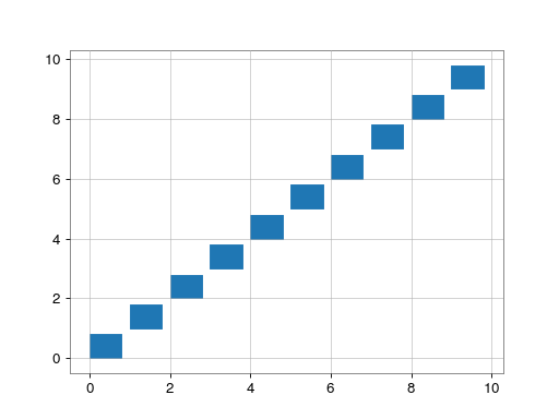