Quickstart#
This quickstart guide will have you analyzing real gravitational-wave data in minutes. We’ll work with public data from the first gravitational-wave detection, GW150914.
What is GWpy?#
The GWpy package contains classes and utilities providing tools and methods for studying data from gravitational-wave detectors, for astrophysical or instrumental purposes.
This package is meant for users who don’t care how the code works necessarily, but want to perform some analysis on some data using a (Python) tool. As a result this package is meant to be as easy-to-use as possible, coupled with extensive documentation of all functions and standard examples of how to use them sensibly.
The core Python infrastructure is influenced by, and extends the functionality of the Astropy package, a superb set of tools for astrophysical analysis.
Additionally, much of the methodology has been derived from, and augmented by,
the LVK Algorithm Library Suite (LALSuite),
a large collection of primarily C99 routines for analysis and manipulation
of data from gravitational-wave detectors.
These packages use the SWIG program to produce Python
wrappings for all C modules, allowing the GWpy package to leverage both the
completeness, and the speed, of these libraries.
In the end, this package has begged, borrowed, and stolen a lot of code from other sources, but should end up packaging them together in a way that makes the whole set easier to use.
Your First GWpy Program#
Let’s start with a complete example, then break it down:
from gwpy.timeseries import TimeSeries

# Download data for GW150914 from LIGO Livingston
data = TimeSeries.get("L1", 1126259446, 1126259478)

# Apply a bandpass filter and whitening to focus on GW signal
filtered = data.bandpass(50, 250).whiten()

# Crop the data to the signal region
cropped = filtered.crop(1126259462, 1126259462.6)

# Create a plot
plot = cropped.plot(
    figsize=(12, 4),
    ylabel="Whitened strain",
    color="gwpy:ligo-livingston",
)
plot.show()
(png)
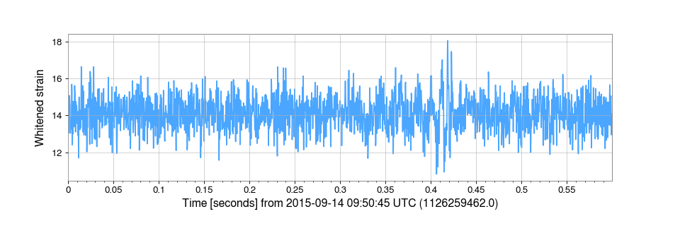
Congratulations! You’ve just analyzed real gravitational-wave data.
Tip
What are those numbers? The numbers 1126259446 and 1126259478
are GPS timestamps marking 32 seconds of data centered on GW150914.
See Key Concepts to learn more about GPS time.
Breaking It Down#
Step 1: Import TimeSeries#
from gwpy.timeseries import TimeSeries
The TimeSeries class is GWpy’s primary data
structure for time-domain data (e.g. detector strain).
Step 2: Download Data#
data = TimeSeries.get("L1", 1126259446, 1126259478)
The TimeSeries.get() method downloads data from a variety of sources
(including GWOSC).
Here we request:
"L1"- data from LIGO Livingston1126259446- start time (GPS seconds)1126259478- end time (GPS seconds)
Step 3: Filter the Data#
filtered = data.bandpass(50, 250).whiten()
cropped = filtered.crop(1126259462, 1126259462.6)
The bandpass() method applies a bandpass filter keeping
frequencies between 50-250 Hz (where gravitational waves are detectable)
and removing low and high frequency noise.
The whiten() method normalises the data to have equal
power at all frequencies, making short signals easier to see.
See also
Signal processing for more on digital filters
The crop() method extracts a smaller time interval
around the signal (from 1126259462 to 1126259462.6 GPS seconds).
Step 4: Make a Plot#
plot = filtered.plot(
    figsize=(12, 4),
    ylabel="Strain amplitude",
    color="gwpy:ligo-livingston",
)
plot.show()
The TimeSeries.plot() method creates a figure with sensible defaults.
We customize:
figsize=(12, 4)- make it wider (12 inches wide by 4 inches high)ylabel="Strain amplitude"- label the Y-axiscolor="gwpy:ligo-livingston"- use LIGO Livingston’s colour
Going Further#
See the Gravitational Wave Signal#
The signal is still hidden in noise. Let’s enhance it by also whitening the data:
from gwpy.timeseries import TimeSeries
# Get data from both LIGO detectors
hdata = TimeSeries.get("H1", 1126259446, 1126259478)
ldata = TimeSeries.get("L1", 1126259446, 1126259478)
# Apply bandpass and whitening to both
hfilt = hdata.bandpass(50, 250).whiten()
lfilt = ldata.bandpass(50, 250).whiten()
# Crop to focus on the signal
hcrop = hfilt.crop(1126259462, 1126259462.6)
lcrop = lfilt.crop(1126259462, 1126259462.6)
# Plot both detectors
from gwpy.plot import Plot
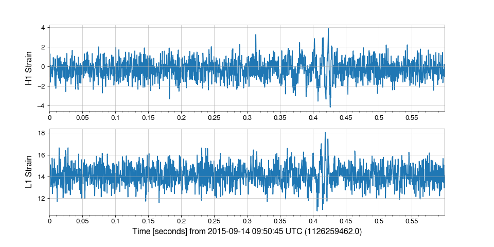
plot = Plot(
hcrop,
lcrop,
figsize=(12, 6),
separate=True,
sharex=True,
)
plot.axes[0].set_ylabel("H1 Strain")
plot.axes[1].set_ylabel("L1 Strain")
plot.show()
(png)

Now you can see the distinctive “chirp” of the gravitational wave signal!
Compute a Q-transform#
Visualize how frequency content changes over time:
from gwpy.timeseries import TimeSeries

data = TimeSeries.get("L1", 1126259446, 1126259478)

# Compute a Q-transform spectrogram, focussing on the signal time
qspecgram = data.q_transform(
    outseg=(1126259462, 1126259462.6),
)

# Plot
plot = qspecgram.plot(figsize=(12, 6))
ax = plot.gca()
ax.set_ylim(20, 500)
ax.colorbar(label="Normalized energy")
plot.show()
(png)
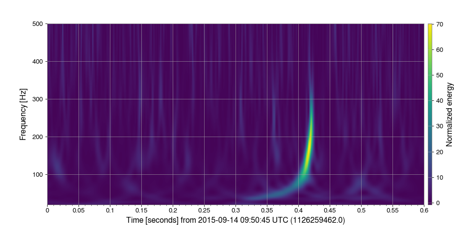
The Q-transform reveals the “chirp” signal increasing in frequency over time!
Calculate a Power Spectrum#
See the detector’s frequency-dependent noise:
from gwpy.timeseries import TimeSeries

data = TimeSeries.get("L1", 1126259446, 1126259478)

# Compute amplitude spectral density
asd = data.asd(fftlength=4, method="median")

# Plot
plot = asd.plot(
    figsize=(12, 6),
    xlabel="Frequency [Hz]",
    xlim=(10, 1200),
    xscale="log",
    ylabel="ASD [strain/√Hz]",
    yscale="log",
    ylim=(2e-24, 1e-19),
)
plot.show()
(png)
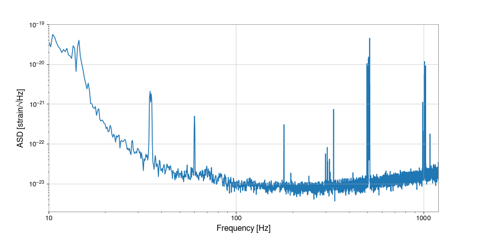
This shows the detector sensitivity curve - lower values mean better sensitivity.
Working with Your Own Data#
Creating TimeSeries from Arrays#
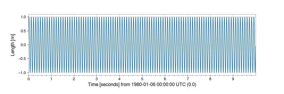
You can create a TimeSeries from any array-like data:
import numpy as np
from gwpy.timeseries import TimeSeries

# Create some sample data
times = np.arange(0, 10, 0.001)  # 10 seconds at 1 kHz
signal = np.sin(2 * np.pi * 10 * times)  # 10 Hz sine wave

# Create a TimeSeries
ts = TimeSeries(signal, sample_rate=1000, t0=0, unit="m")

print(ts)
plot = ts.plot()
plot.show()
(png)

Reading from Files#
GWpy can read many file formats:
from gwpy.timeseries import TimeSeries

# Read from HDF5
data = TimeSeries.read("mydata.h5", channel="L1:GDS-CALIB_STRAIN")

# Read from GWF (requires lalframe)
data = TimeSeries.read("L-L1_GWOSC_4KHZ_R1-1126259447-32.gwf")
See also
Reading and writing time series data for all supported formats
Next Steps#
Now that you’ve completed the quickstart, you’re ready to dive deeper:
Understand TimeSeries, GPS time, and other key concepts
Task-focused guides for common operations
Gallery of working code examples
Getting Help#
Documentation: You’re in it! Use the search box above.
Slack: Join our community Slack for questions
Issues: Report bugs on our GitLab issue tracker
Email: For private inquiries, contact the maintainers
See also
Key Concepts - Core GWpy concepts explained
User Guide - User Guide
API Reference - Complete API reference